Normative

The five sequences—Nihilism through Integration, Lens, Fragmented to United, Hate to Trust, and Cacophony to Symphony—provide a framework to examine ethical data sharing within the clinical research ecosystem, particularly through a web app for living donor nephrectomy decisions that bypasses IRB inefficiencies. This ecosystem, comprising students, professors, care providers, patients, analysts, academic departments, administrators, and federal employees with NHANES access, generates Kaplan-Meier curves from donor and NHANES data to assess outcomes like perioperative mortality or ESRD risk. By using clear GitHub workflows—public repositories for de-identified data and private ones for identified data, distinctly labeled—each sequence reveals how ethical data sharing can balance transparency, accountability, and efficiency while safeguarding privacy and trust.

Fig. 39 I’d advise you to consider your position carefully (layer 3 fork in the road), perhaps adopting a more flexible posture (layer 4 dynamic capabilities realized), while keeping your ear to the ground (layer 2 yellow node), covering your retreat (layer 5 Athena’s shield, helmet, and horse), and watching your rear (layer 1 ecosystem and perspective).

The first sequence, Nihilism to Integration, casts ethical data sharing as a journey from ethical lapse to principled unity. Nihilism, a failure to integrate, emerges when data hoarding or reckless sharing violates ethics: a professor withholds donor stats, risking incomplete risk curves, or an analyst leaks identified NHANES records. Deconstruction exposes these breaches—labeling data as “de-id_risk” or “id_patient” clarifies boundaries. Perspective arises as stakeholders prioritize consent and privacy, using GitHub’s public-private split to share responsibly. Awareness drives ethical protocols—de-identified NHANES goes public, identified donor data stays private with access logs. Reconstruction builds the app’s back end, harmonizing data under these rules, and Integration delivers a tool where 95% CIs reflect ethically sourced inputs. This arc shows ethical sharing as integration’s cornerstone, replacing IRB delays with self-imposed rigor.

“Lens,” the second sequence, is the web app—a nexus where ethical sharing crystallizes. Hosted on GitHub Pages, it merges de-identified NHANES baselines (publicly labeled “de-id_cum_inc”) with private donor coefficients (tagged “private_beta”), ensuring patients see only anonymized curves via drop-down inputs. Analysts share models ethically by restricting identified data to authorized collaborators, while professors validate outputs without exposing raw records. Sparse data—like for elderly donors—widens CIs, but transparency about this limitation (e.g., “low_n_flag”) upholds integrity. Bypassing IRB, the Lens relies on clear labeling and access controls to maintain ethics: public data educates, private data protects, proving that ethical sharing can thrive outside traditional oversight when workflows enforce accountability.

Fragmented to United, the third sequence, reflects ethical sharing’s role in unifying the ecosystem. Fragmentation risks ethics violations—unshared NHANES controls skew curves, or unlabeled donor data leaks identifiable details. GitHub workflows counter this: public repos offer de-identified aggregates for all, private ones limit identified records to vetted users (e.g., “id_access:careprovider1”). This unites stakeholders—patients trust anonymized risks, analysts rely on harmonized inputs—without IRB lag. The challenge lies in consistency: mislabeled data (e.g., “de-id” with hidden identifiers) breaches ethics, widening mistrust. When executed well, this sequence shows ethical sharing as a unifying force, aligning fragmented parts into a safe, shared truth.

The fourth sequence, Hate to Trust, navigates the ethical tensions of data sharing. “Hate” flares as fear—patients dread privacy breaches, administrators foresee lawsuits, federal employees guard NHANES against misuse. “Negotiate” balances this: public de-identified data (e.g., “de-id_mortality”) is freely shared, while private identified data (e.g., “id_event_time”) requires consent and restricted access, logged on GitHub. “Trust” emerges as ethical sharing holds—patients see reliable curves, care providers counsel with confidence, and professors publish without compromising sources. This dynamic underscores ethics as a trust pact: bypassing IRB demands rigorous self-regulation—labeling, anonymization, audit trails—to replace external rules with internal integrity, ensuring data serves without harm.

Cacophony to Symphony, the fifth sequence, harmonizes the ethical cacophony of data sharing. “Cacophony” erupts from ethical noise—unlabeled donor risks, NHANES privacy debates, analysts’ unchecked tweaks—threatening chaos. “Outside” sees public NHANES data shared ethically, stripped of identifiers, while “Emotion” captures stakes: patients’ vulnerability, students’ duty to learn responsibly. “Inside” refines this via private repos, where identified data (e.g., “id_periop_outcome”) is siloed yet ethically linked to de-identified outputs. “Symphony” rings true as the app integrates these—curves reflect a balance of openness and protection, stakeholders align in trust. This arc proves ethical sharing turns discord into harmony, using workflows to enforce privacy while maximizing utility.

Ethical data sharing, as seen here, hinges on transparency and discipline—GitHub’s public-private split, clear labels like “de-id” vs. “id,” and consent-driven access. The app, bypassing IRB, shows this can work: de-identified NHANES educates broadly, identified donor data informs precisely, and the ecosystem thrives without leaks or delays. Beyond medicine—think open-source tech or policy analytics—this scales where workflows replace bureaucracy, balancing ethics with efficiency. The risk is human slip—mislabeling or over-sharing—but the reward is an agile, trustworthy system, proving ethics need not slow progress when baked into the process itself.

Show code cell source Hide code cell source

import numpy as np
import matplotlib.pyplot as plt
import networkx as nx

# Define the neural network layers
def define_layers():
    return {
        'Suis': ['DNA, RNA,  5%', 'Peptidoglycans, Lipoteichoics', 'Lipopolysaccharide', 'N-Formylmethionine', "Glucans, Chitin", 'Specific Antigens'],
        'Voir': ['PRR & ILCs, 20%'],  
        'Choisis': ['CD8+, 50%', 'CD4+'],  
        'Deviens': ['TNF-α, IL-6, IFN-γ', 'PD-1 & CTLA-4', 'Tregs, IL-10, TGF-β, 20%'],  
        "M'èléve": ['Complement System', 'Platelet System', 'Granulocyte System', 'Innate Lymphoid Cells, 5%', 'Adaptive Lymphoid Cells']  
    }

# Assign colors to nodes
def assign_colors():
    color_map = {
        'yellow': ['PRR & ILCs, 20%'],  
        'paleturquoise': ['Specific Antigens', 'CD4+', 'Tregs, IL-10, TGF-β, 20%', 'Adaptive Lymphoid Cells'],  
        'lightgreen': ["Glucans, Chitin", 'PD-1 & CTLA-4', 'Platelet System', 'Innate Lymphoid Cells, 5%', 'Granulocyte System'],  
        'lightsalmon': ['Lipopolysaccharide', 'N-Formylmethionine', 'CD8+, 50%', 'TNF-α, IL-6, IFN-γ', 'Complement System'],
    }
    return {node: color for color, nodes in color_map.items() for node in nodes}

# Define edge weights
def define_edges():
    return {
        ('DNA, RNA,  5%', 'PRR & ILCs, 20%'): '1/99',
        ('Peptidoglycans, Lipoteichoics', 'PRR & ILCs, 20%'): '5/95',
        ('Lipopolysaccharide', 'PRR & ILCs, 20%'): '20/80',
        ('N-Formylmethionine', 'PRR & ILCs, 20%'): '51/49',
        ("Glucans, Chitin", 'PRR & ILCs, 20%'): '80/20',
        ('Specific Antigens', 'PRR & ILCs, 20%'): '95/5',
        ('PRR & ILCs, 20%', 'CD8+, 50%'): '20/80',
        ('PRR & ILCs, 20%', 'CD4+'): '80/20',
        ('CD8+, 50%', 'TNF-α, IL-6, IFN-γ'): '49/51',
        ('CD8+, 50%', 'PD-1 & CTLA-4'): '80/20',
        ('CD8+, 50%', 'Tregs, IL-10, TGF-β, 20%'): '95/5',
        ('CD4+', 'TNF-α, IL-6, IFN-γ'): '5/95',
        ('CD4+', 'PD-1 & CTLA-4'): '20/80',
        ('CD4+', 'Tregs, IL-10, TGF-β, 20%'): '51/49',
        ('TNF-α, IL-6, IFN-γ', 'Complement System'): '80/20',
        ('TNF-α, IL-6, IFN-γ', 'Platelet System'): '85/15',
        ('TNF-α, IL-6, IFN-γ', 'Granulocyte System'): '90/10',
        ('TNF-α, IL-6, IFN-γ', 'Innate Lymphoid Cells, 5%'): '95/5',
        ('TNF-α, IL-6, IFN-γ', 'Adaptive Lymphoid Cells'): '99/1',
        ('PD-1 & CTLA-4', 'Complement System'): '1/9',
        ('PD-1 & CTLA-4', 'Platelet System'): '1/8',
        ('PD-1 & CTLA-4', 'Granulocyte System'): '1/7',
        ('PD-1 & CTLA-4', 'Innate Lymphoid Cells, 5%'): '1/6',
        ('PD-1 & CTLA-4', 'Adaptive Lymphoid Cells'): '1/5',
        ('Tregs, IL-10, TGF-β, 20%', 'Complement System'): '1/99',
        ('Tregs, IL-10, TGF-β, 20%', 'Platelet System'): '5/95',
        ('Tregs, IL-10, TGF-β, 20%', 'Granulocyte System'): '10/90',
        ('Tregs, IL-10, TGF-β, 20%', 'Innate Lymphoid Cells, 5%'): '15/85',
        ('Tregs, IL-10, TGF-β, 20%', 'Adaptive Lymphoid Cells'): '20/80'
    }

# Define edges to be highlighted in black
def define_black_edges():
    return {
        ('PRR & ILCs, 20%', 'CD4+'): '80/20',
        ('CD4+', 'TNF-α, IL-6, IFN-γ'): '5/95',
        ('CD4+', 'PD-1 & CTLA-4'): '20/80',
        ('CD4+', 'Tregs, IL-10, TGF-β, 20%'): '51/49',
    }

# Calculate node positions
def calculate_positions(layer, x_offset):
    y_positions = np.linspace(-len(layer) / 2, len(layer) / 2, len(layer))
    return [(x_offset, y) for y in y_positions]

# Create and visualize the neural network graph
def visualize_nn():
    layers = define_layers()
    colors = assign_colors()
    edges = define_edges()
    black_edges = define_black_edges()
    
    G = nx.DiGraph()
    pos = {}
    node_colors = []
    
    # Create mapping from original node names to numbered labels
    mapping = {}
    counter = 1
    for layer in layers.values():
        for node in layer:
            mapping[node] = f"{counter}. {node}"
            counter += 1
            
    # Add nodes with new numbered labels and assign positions
    for i, (layer_name, nodes) in enumerate(layers.items()):
        positions = calculate_positions(nodes, x_offset=i * 2)
        for node, position in zip(nodes, positions):
            new_node = mapping[node]
            G.add_node(new_node, layer=layer_name)
            pos[new_node] = position
            node_colors.append(colors.get(node, 'lightgray'))
    
    # Add edges with updated node labels
    edge_colors = []
    for (source, target), weight in edges.items():
        if source in mapping and target in mapping:
            new_source = mapping[source]
            new_target = mapping[target]
            G.add_edge(new_source, new_target, weight=weight)
            edge_colors.append('black' if (source, target) in black_edges else 'lightgrey')
    
    # Draw the graph
    plt.figure(figsize=(12, 8))
    edges_labels = {(u, v): d["weight"] for u, v, d in G.edges(data=True)}
    
    nx.draw(
        G, pos, with_labels=True, node_color=node_colors, edge_color=edge_colors,
        node_size=3000, font_size=9, connectionstyle="arc3,rad=0.2"
    )
    nx.draw_networkx_edge_labels(G, pos, edge_labels=edges_labels, font_size=8)
    plt.title("OPRAH™: Nonself & the Salient Network", fontsize=18)
    plt.show()

# Run the visualization
visualize_nn()

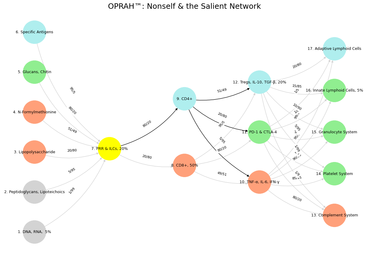
Fig. 40 Space is Apollonian and Time Dionysian. They are the static representation and the dynamic emergent. Ain’t that somethin?