Freedom in Fetters

The five sequences—Nihilism through Integration, Lens, Fragmented to United, Hate to Trust, and Cacophony to Symphony—cast a revealing light on the challenges of data integration within the clinical research ecosystem, as embodied by a web app for living donor nephrectomy decisions. This ecosystem, linking students, professors, care providers, patients, analysts, academic departments, administrators, and federal employees with NHANES access, relies on integrating diverse data—donor registries, NHANES controls, Cox regression outputs—to power Kaplan-Meier curves for outcomes like perioperative mortality or ESRD risk. Each sequence highlights distinct hurdles in this process, from siloed mindsets to technical mismatches, exposing the friction that threatens the app’s efficacy and the ecosystem’s cohesion.

Fig. 30 The five networks described in the essay, mapped to Uganda’s and Africa’s identity negotiation, unfold as follows: First, the Pericentral network (sensory-motor) governs reflexive responses, reacting to “nonself” threats like colonialism with immediate, physical action. Second, the Dorsal Frontoparietal network (goal-directed attention) focuses on detecting and prioritizing nonself entities, potentially faltering in Africa’s blurred boundaries with foreign influence. Third, the Lateral Frontoparietal network (flexible decision-making) navigates ambiguity, reflecting the continent’s struggle to balance tribal diversity and imposed systems. Fourth, the Medial Frontoparietal network (self-referential identity) turns inward, emphasizing self-coherence over external rejection, perhaps overly so in Africa’s history. Fifth, the Cingulo-Insular network (salience optimization) integrates these, ideally balancing self and nonself for efficiency—a convergence Africa might yet achieve. The order—from reflex to attention, ambiguity, identity, and optimization—mirrors a progression from instinctive reaction to reflective synthesis, suggesting a natural arc of development, though not necessarily a hierarchy; Africa’s “error” may lie in stalling at ambiguity or self-focus, short of full convergence.

The first sequence, Nihilism to Integration, frames data integration as a battle against disintegration. Nihilism, a failure to integrate, surfaces when data remains trapped: a professor’s IRB-approved donor dataset sits unshared, an analyst’s variance-covariance matrix stays local, or NHANES controls are inaccessible behind bureaucratic walls. Deconstruction reveals the problem—disparate formats (e.g., .csv vs. proprietary files) or incompatible ethics protocols thwart merging. Perspective shows the scale: stakeholders see how unintegrated data skews the app’s 95% CIs, like wild estimates for an 85-year-old donor due to sparse records. Awareness of this gap drives Reconstruction, but challenges persist—standardizing NHANES baselines with donor stats demands time and skill. Integration, the app’s back end on GitHub Pages, succeeds only if these barriers are overcome, underscoring a core challenge: data’s value hinges on conquering isolation, a task easier envisioned than executed.

“Lens,” the second sequence, is the web app—a fragile hub where integration challenges converge. Built with JavaScript and HTML, it aims to fuse a .csv file of beta coefficients, NHANES cumulative incidence functions, and patient inputs from drop-down menus. Yet, heterogeneity bites: donor data might use different time scales than NHANES, or analysts’ Cox models clash with federal parametric assumptions. Patients expect seamless curves, but sparse data—say, for elderly donors—widens CIs, exposing gaps in the integrated set. Administrators face IRB hurdles to align consent across sources, while professors and analysts wrestle with versioning on GitHub. The Lens reveals integration’s technical crux: disparate data must be normalized and synced, a process rife with mismatches that threaten the app’s clarity and trust.

Fragmented to United, the third sequence, spotlights integration’s binary tension. Fragmentation reigns when data sources don’t speak—NHANES controls lack donor-specific granularity, or student analyses miss clinical context. The app’s two curves (baseline vs. nephrectomy) demand a unified dataset, but incomplete integration—missing elderly donor outcomes or unmerged registries—undermines precision. Care providers need reliable risks, yet fragmented inputs yield shaky outputs. Uniting this requires metadata alignment, a Herculean task when departments guard their schemas or federal employees limit access. This sequence lays bare a structural challenge: integration falters without shared standards, leaving the ecosystem split between potential and reality.

The fourth sequence, Hate to Trust, uncovers the human and ethical roadblocks to integration. “Hate” emerges as resistance—patients fear unintegrated data misrepresents their risk, analysts distrust professors’ unshared adjustments, or administrators balk at exposing sensitive NHANES extracts. “Negotiate” is the fraught compromise: a federal employee anonymizes controls, a professor releases partial stats, but misaligned priorities (publication vs. utility) stall progress. “Trust” hinges on integration’s success—stakeholders embrace the app only if its curves reflect a cohesive truth, not a patchwork of half-merged inputs. This dynamic exposes a relational challenge: data integration requires consensus on ownership and use, a negotiation often derailed by mistrust or legal red tape.

Cacophony to Symphony, the fifth sequence, amplifies the chaotic clash of integration efforts. “Cacophony” is the noise—unstandardized donor records, NHANES outliers, analysts’ competing regression tweaks—drowning out coherence. “Outside” highlights external data’s incompatibility, like NHANES’ broad population clashing with donor specifics. “Emotion” captures the fallout: frustration as students debug mismatches, anxiety as patients face uncertain curves. “Inside” is the app’s attempt to reconcile this—a base-case function strained by gaps—while “Symphony” demands a miracle: harmonizing discordant sources into reliable outputs. This sequence reveals integration’s practical mess: data’s diversity, from formats to quality, resists unification, testing the ecosystem’s patience and tools.

These challenges—silos, technical disparity, standardization, trust, and chaos—plague any data-driven ecosystem, from healthcare to tech. The nephrectomy app, reliant on GitHub-shared scripts and a .csv backbone, shows integration’s stakes: success empowers decisions, but failure breeds doubt. Bridging NHANES to donor data or analysts to patients tests the ecosystem’s resilience, proving integration is less a technical fix than a collective triumph over fragmentation’s inertia.

Show code cell source Hide code cell source

import numpy as np
import matplotlib.pyplot as plt
import networkx as nx

# Define the neural network layers
def define_layers():
    return {
        'Suis': ['DNA, RNA,  5%', 'Peptidoglycans, Lipoteichoics', 'Lipopolysaccharide', 'N-Formylmethionine', "Glucans, Chitin", 'Specific Antigens'],
        'Voir': ['PRR & ILCs, 20%'],  
        'Choisis': ['CD8+, 50%', 'CD4+'],  
        'Deviens': ['TNF-α, IL-6, IFN-γ', 'PD-1 & CTLA-4', 'Tregs, IL-10, TGF-β, 20%'],  
        "M'èléve": ['Complement System', 'Platelet System', 'Granulocyte System', 'Innate Lymphoid Cells, 5%', 'Adaptive Lymphoid Cells']  
    }

# Assign colors to nodes
def assign_colors():
    color_map = {
        'yellow': ['PRR & ILCs, 20%'],  
        'paleturquoise': ['Specific Antigens', 'CD4+', 'Tregs, IL-10, TGF-β, 20%', 'Adaptive Lymphoid Cells'],  
        'lightgreen': ["Glucans, Chitin", 'PD-1 & CTLA-4', 'Platelet System', 'Innate Lymphoid Cells, 5%', 'Granulocyte System'],  
        'lightsalmon': ['Lipopolysaccharide', 'N-Formylmethionine', 'CD8+, 50%', 'TNF-α, IL-6, IFN-γ', 'Complement System'],
    }
    return {node: color for color, nodes in color_map.items() for node in nodes}

# Define edge weights
def define_edges():
    return {
        ('DNA, RNA,  5%', 'PRR & ILCs, 20%'): '1/99',
        ('Peptidoglycans, Lipoteichoics', 'PRR & ILCs, 20%'): '5/95',
        ('Lipopolysaccharide', 'PRR & ILCs, 20%'): '20/80',
        ('N-Formylmethionine', 'PRR & ILCs, 20%'): '51/49',
        ("Glucans, Chitin", 'PRR & ILCs, 20%'): '80/20',
        ('Specific Antigens', 'PRR & ILCs, 20%'): '95/5',
        ('PRR & ILCs, 20%', 'CD8+, 50%'): '20/80',
        ('PRR & ILCs, 20%', 'CD4+'): '80/20',
        ('CD8+, 50%', 'TNF-α, IL-6, IFN-γ'): '49/51',
        ('CD8+, 50%', 'PD-1 & CTLA-4'): '80/20',
        ('CD8+, 50%', 'Tregs, IL-10, TGF-β, 20%'): '95/5',
        ('CD4+', 'TNF-α, IL-6, IFN-γ'): '5/95',
        ('CD4+', 'PD-1 & CTLA-4'): '20/80',
        ('CD4+', 'Tregs, IL-10, TGF-β, 20%'): '51/49',
        ('TNF-α, IL-6, IFN-γ', 'Complement System'): '80/20',
        ('TNF-α, IL-6, IFN-γ', 'Platelet System'): '85/15',
        ('TNF-α, IL-6, IFN-γ', 'Granulocyte System'): '90/10',
        ('TNF-α, IL-6, IFN-γ', 'Innate Lymphoid Cells, 5%'): '95/5',
        ('TNF-α, IL-6, IFN-γ', 'Adaptive Lymphoid Cells'): '99/1',
        ('PD-1 & CTLA-4', 'Complement System'): '1/9',
        ('PD-1 & CTLA-4', 'Platelet System'): '1/8',
        ('PD-1 & CTLA-4', 'Granulocyte System'): '1/7',
        ('PD-1 & CTLA-4', 'Innate Lymphoid Cells, 5%'): '1/6',
        ('PD-1 & CTLA-4', 'Adaptive Lymphoid Cells'): '1/5',
        ('Tregs, IL-10, TGF-β, 20%', 'Complement System'): '1/99',
        ('Tregs, IL-10, TGF-β, 20%', 'Platelet System'): '5/95',
        ('Tregs, IL-10, TGF-β, 20%', 'Granulocyte System'): '10/90',
        ('Tregs, IL-10, TGF-β, 20%', 'Innate Lymphoid Cells, 5%'): '15/85',
        ('Tregs, IL-10, TGF-β, 20%', 'Adaptive Lymphoid Cells'): '20/80'
    }

# Define edges to be highlighted in black
def define_black_edges():
    return {
        ('DNA, RNA,  5%', 'PRR & ILCs, 20%'): '1/99',
        ('Peptidoglycans, Lipoteichoics', 'PRR & ILCs, 20%'): '5/95',
        ('Lipopolysaccharide', 'PRR & ILCs, 20%'): '20/80',
        ('N-Formylmethionine', 'PRR & ILCs, 20%'): '51/49',
        ("Glucans, Chitin", 'PRR & ILCs, 20%'): '80/20',
        ('Specific Antigens', 'PRR & ILCs, 20%'): '95/5',
    }

# Calculate node positions
def calculate_positions(layer, x_offset):
    y_positions = np.linspace(-len(layer) / 2, len(layer) / 2, len(layer))
    return [(x_offset, y) for y in y_positions]

# Create and visualize the neural network graph
def visualize_nn():
    layers = define_layers()
    colors = assign_colors()
    edges = define_edges()
    black_edges = define_black_edges()
    
    G = nx.DiGraph()
    pos = {}
    node_colors = []
    
    # Create mapping from original node names to numbered labels
    mapping = {}
    counter = 1
    for layer in layers.values():
        for node in layer:
            mapping[node] = f"{counter}. {node}"
            counter += 1
            
    # Add nodes with new numbered labels and assign positions
    for i, (layer_name, nodes) in enumerate(layers.items()):
        positions = calculate_positions(nodes, x_offset=i * 2)
        for node, position in zip(nodes, positions):
            new_node = mapping[node]
            G.add_node(new_node, layer=layer_name)
            pos[new_node] = position
            node_colors.append(colors.get(node, 'lightgray'))
    
    # Add edges with updated node labels
    edge_colors = []
    for (source, target), weight in edges.items():
        if source in mapping and target in mapping:
            new_source = mapping[source]
            new_target = mapping[target]
            G.add_edge(new_source, new_target, weight=weight)
            edge_colors.append('black' if (source, target) in black_edges else 'lightgrey')
    
    # Draw the graph
    plt.figure(figsize=(12, 8))
    edges_labels = {(u, v): d["weight"] for u, v, d in G.edges(data=True)}
    
    nx.draw(
        G, pos, with_labels=True, node_color=node_colors, edge_color=edge_colors,
        node_size=3000, font_size=9, connectionstyle="arc3,rad=0.2"
    )
    nx.draw_networkx_edge_labels(G, pos, edge_labels=edges_labels, font_size=8)
    plt.title("OPRAH™ aAPCs", fontsize=18)
    plt.show()

# Run the visualization
visualize_nn()

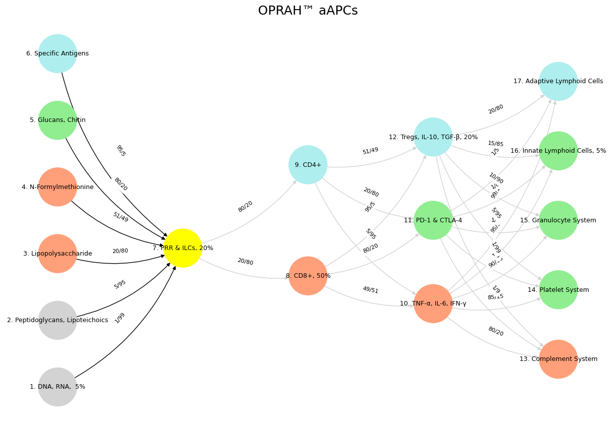
Fig. 31 Musical Grammar & Prosody. From a pianist’s perspective, the left hand serves as the foundational architect, voicing the mode and defining the musical landscape—its space and grammar—while the right hand acts as the expressive wanderer, freely extending and altering these modal terrains within temporal pockets, guided by prosody and cadence. In R&B, this interplay often manifests through rich harmonic extensions like 9ths, 11ths, and 13ths, with chromatic passing chords and leading tones adding tension and color. Music’s evocative power lies in its ability to transmit information through a primal, pattern-recognizing architecture, compelling listeners to classify what they hear as either nurturing or threatening—feeding and breeding or fight and flight. This makes music a high-risk, high-reward endeavor, where success hinges on navigating the fine line between coherence and error. Similarly, pattern recognition extends to literature, as seen in Ulysses, where a character misinterprets his companion’s silence as mental composition, reflecting on the instructive pleasures of Shakespearean works used to solve life’s complexities. Both music and literature, then, are deeply rooted in the human impulse to decode and derive meaning, whether through harmonic landscapes or textual introspection. Source: Ulysses, DeepSeek & Yours Truly!