Transvaluation

The five sequences—Nihilism through Integration, Lens, Fragmented to United, Hate to Trust, and Cacophony to Symphony—offer a lens into ecosystem dynamics when viewed through the context of clinical research and a decision-making web app for living donor nephrectomy. Here, the ecosystem is the scientific enterprise: a sprawling network of students, professors, care providers, patients, analysts, academic departments, administrators, and federal data stewards, all interacting within the flow of data, ethics, and outcomes. The sequences illuminate how this ecosystem grapples with integration, navigation, and the tension between chaos and coherence, revealing broader principles of how such systems function, adapt, and thrive—or falter.

Fig. 23 Salient Network: Midcingulo-Insular Network. The framework’s real limit is its refusal to admit how shallow these parallels run—immune and neural systems don’t “converge” beyond basic problem-solving, and dressing them in tech jargon doesn’t deepen the link. OPRAH™ maps a compelling comparison, but its sharpness cuts only skin-deep, leaving the messy guts of biology untouched.

The first sequence, Nihilism to Integration, frames ecosystem dynamics as a struggle for cohesion. Nihilism, defined as a failure to integrate, marks the ecosystem’s low point: data silos (e.g., NHANES controls separate from donor registries), misaligned incentives (researchers vs. clinicians), or unshared tools (an analyst’s Python script sitting idle). Deconstruction dismantles these barriers—think of a professor sharing IRB-approved data via GitHub—exposing the system’s fractures. Perspective emerges as stakeholders recognize their interdependence, like a student seeing how their input fits a larger study. Awareness dawns with the realization of potential synergy, driving Reconstruction: a collaborative push to align efforts, perhaps coding the web app’s back end with Cox regression outputs. Integration completes the cycle, binding the ecosystem into a unified whole—the app itself, hosted on GitHub Pages, where patients and providers draw from the same .csv file. This arc reveals a core dynamic: ecosystems stagnate in isolation but evolve through deliberate reconnection.

“Lens,” the second sequence, embodies the ecosystem’s focal mechanism—the web app accessed via QR code. It’s not just a tool but a dynamic node, channeling interactions via JavaScript, HTML, and a beta coefficient vector. Students tweak drop-down menus, analysts refine variance-covariance matrices, and patients interpret Kaplan-Meier curves for perioperative mortality or ESRD risk, all within its interactive framework. The Lens reflects an ecosystem’s need for a shared interface: it absorbs inputs (demographic data), processes uncertainty (wide CIs for an 85-year-old donor), and outputs clarity (two curves, baseline vs. decision). Its role highlights a key dynamic: ecosystems rely on adaptive hubs—here, a simple app—that balance flexibility and structure, enabling navigation amid complexity.

Fragmented to United, the third sequence, captures the ecosystem’s binary pulse. The stark choice between two curves (no donation vs. nephrectomy) mirrors its constant oscillation between disorder and synthesis. Fragmentation reigns when data sources (NHANES, donor registries) or actors (departments, patients) operate in silos, like unlinked roots in a forest. United emerges when the Lens integrates them, aligning disparate strands into a single decision point. This dynamic underscores an ecosystem’s resilience: it thrives by bridging divides, turning scattered inputs into collective action, much as a clinician’s choice reflects the labor of unseen analysts and administrators.

The fourth sequence, Hate to Trust, maps the ecosystem’s transactional heartbeat. “Hate” symbolizes friction—adverse outcomes (perioperative death, long-term ESRD) or mistrust in sparse data (wild CIs). “Negotiate” is the bargaining: weighing donor risks against recipient benefits or waitlist reduction, a dance of trade-offs mediated by informed consent. “Trust” arises as the ecosystem stabilizes—patients rely on the app’s curves, providers on its evidence, and analysts on shared code. This progression reveals a relational dynamic: ecosystems are sustained by negotiation, where conflicting interests (safety vs. altruism) resolve into mutual dependence, lubricated by tools like the Lens.

Cacophony to Symphony, the fifth sequence, portrays the ecosystem’s sensory and synthetic flow. Cacophony erupts from its noise—competing voices (patients’ fears, professors’ hypotheses), raw data (missed workdays, 30-year mortality risks), and external pressures (IRB delays). “Outside” shifts focus to the ecosystem’s edges—NHANES controls or federal employees—while “Emotion” internalizes this chaos, as stakeholders feel the weight of decisions. “Inside” is the app’s distillation, processing inputs into curves, and “Symphony” is the harmony of resolution: a patient’s informed choice, a researcher’s validated model. This arc exposes a vital dynamic: ecosystems metabolize disorder into order, cycling external inputs through internal synthesis, with tools like the app acting as catalysts.

These dynamics generalize beyond clinical research. In any ecosystem—be it a tech startup, a city, or a family—Nihilism’s disintegration looms when parts fail to connect (unshared resources, miscommunication). A Lens (an app, a leader, a rule) focuses effort, uniting Fragmented elements into a binary clarity (act or don’t). Hate-to-Trust negotiates stakes (profit vs. ethics, growth vs. stability), while Cacophony-to-Symphony transforms noise (conflicting goals, data overload) into coherence. The nephrectomy app, born from a Stata script and GitHub collaboration, exemplifies this: a fragile ecosystem of science integrates via a simple interface, navigates uncertainty, and empowers decisions. Its power lies in revealing how ecosystems, medical or otherwise, dance between collapse and creation, driven by the interplay of their parts.

Show code cell source Hide code cell source

import numpy as np
import matplotlib.pyplot as plt
import networkx as nx

# Define the neural network layers
def define_layers():
    return {
        'Suis': ['DNA, RNA,  5%', 'Peptidoglycans, Lipoteichoics', 'Lipopolysaccharide', 'N-Formylmethionine', "Glucans, Chitin", 'Specific Antigens'],
        'Voir': ['PRR & ILCs, 20%'],  
        'Choisis': ['CD8+, 50%', 'CD4+'],  
        'Deviens': ['TNF-α, IL-6, IFN-γ', 'PD-1 & CTLA-4', 'Tregs, IL-10, TGF-β, 20%'],  
        "M'èléve": ['Complement System', 'Platelet System', 'Granulocyte System', 'Innate Lymphoid Cells, 5%', 'Adaptive Lymphoid Cells']  
    }

# Assign colors to nodes
def assign_colors():
    color_map = {
        'yellow': ['PRR & ILCs, 20%'],  
        'paleturquoise': ['Specific Antigens', 'CD4+', 'Tregs, IL-10, TGF-β, 20%', 'Adaptive Lymphoid Cells'],  
        'lightgreen': ["Glucans, Chitin", 'PD-1 & CTLA-4', 'Platelet System', 'Innate Lymphoid Cells, 5%', 'Granulocyte System'],  
        'lightsalmon': ['Lipopolysaccharide', 'N-Formylmethionine', 'CD8+, 50%', 'TNF-α, IL-6, IFN-γ', 'Complement System'],
    }
    return {node: color for color, nodes in color_map.items() for node in nodes}

# Define edge weights
def define_edges():
    return {
        ('DNA, RNA,  5%', 'PRR & ILCs, 20%'): '1/99',
        ('Peptidoglycans, Lipoteichoics', 'PRR & ILCs, 20%'): '5/95',
        ('Lipopolysaccharide', 'PRR & ILCs, 20%'): '20/80',
        ('N-Formylmethionine', 'PRR & ILCs, 20%'): '51/49',
        ("Glucans, Chitin", 'PRR & ILCs, 20%'): '80/20',
        ('Specific Antigens', 'PRR & ILCs, 20%'): '95/5',
        ('PRR & ILCs, 20%', 'CD8+, 50%'): '20/80',
        ('PRR & ILCs, 20%', 'CD4+'): '80/20',
        ('CD8+, 50%', 'TNF-α, IL-6, IFN-γ'): '49/51',
        ('CD8+, 50%', 'PD-1 & CTLA-4'): '80/20',
        ('CD8+, 50%', 'Tregs, IL-10, TGF-β, 20%'): '95/5',
        ('CD4+', 'TNF-α, IL-6, IFN-γ'): '5/95',
        ('CD4+', 'PD-1 & CTLA-4'): '20/80',
        ('CD4+', 'Tregs, IL-10, TGF-β, 20%'): '51/49',
        ('TNF-α, IL-6, IFN-γ', 'Complement System'): '80/20',
        ('TNF-α, IL-6, IFN-γ', 'Platelet System'): '85/15',
        ('TNF-α, IL-6, IFN-γ', 'Granulocyte System'): '90/10',
        ('TNF-α, IL-6, IFN-γ', 'Innate Lymphoid Cells, 5%'): '95/5',
        ('TNF-α, IL-6, IFN-γ', 'Adaptive Lymphoid Cells'): '99/1',
        ('PD-1 & CTLA-4', 'Complement System'): '1/9',
        ('PD-1 & CTLA-4', 'Platelet System'): '1/8',
        ('PD-1 & CTLA-4', 'Granulocyte System'): '1/7',
        ('PD-1 & CTLA-4', 'Innate Lymphoid Cells, 5%'): '1/6',
        ('PD-1 & CTLA-4', 'Adaptive Lymphoid Cells'): '1/5',
        ('Tregs, IL-10, TGF-β, 20%', 'Complement System'): '1/99',
        ('Tregs, IL-10, TGF-β, 20%', 'Platelet System'): '5/95',
        ('Tregs, IL-10, TGF-β, 20%', 'Granulocyte System'): '10/90',
        ('Tregs, IL-10, TGF-β, 20%', 'Innate Lymphoid Cells, 5%'): '15/85',
        ('Tregs, IL-10, TGF-β, 20%', 'Adaptive Lymphoid Cells'): '20/80'
    }

# Define edges to be highlighted in black
def define_black_edges():
    return {
        ('DNA, RNA,  5%', 'PRR & ILCs, 20%'): '1/99',
        ('Peptidoglycans, Lipoteichoics', 'PRR & ILCs, 20%'): '5/95',
        ('Lipopolysaccharide', 'PRR & ILCs, 20%'): '20/80',
        ('N-Formylmethionine', 'PRR & ILCs, 20%'): '51/49',
        ("Glucans, Chitin", 'PRR & ILCs, 20%'): '80/20',
        ('Specific Antigens', 'PRR & ILCs, 20%'): '95/5',
    }

# Calculate node positions
def calculate_positions(layer, x_offset):
    y_positions = np.linspace(-len(layer) / 2, len(layer) / 2, len(layer))
    return [(x_offset, y) for y in y_positions]

# Create and visualize the neural network graph
def visualize_nn():
    layers = define_layers()
    colors = assign_colors()
    edges = define_edges()
    black_edges = define_black_edges()
    
    G = nx.DiGraph()
    pos = {}
    node_colors = []
    
    # Create mapping from original node names to numbered labels
    mapping = {}
    counter = 1
    for layer in layers.values():
        for node in layer:
            mapping[node] = f"{counter}. {node}"
            counter += 1
            
    # Add nodes with new numbered labels and assign positions
    for i, (layer_name, nodes) in enumerate(layers.items()):
        positions = calculate_positions(nodes, x_offset=i * 2)
        for node, position in zip(nodes, positions):
            new_node = mapping[node]
            G.add_node(new_node, layer=layer_name)
            pos[new_node] = position
            node_colors.append(colors.get(node, 'lightgray'))
    
    # Add edges with updated node labels
    edge_colors = []
    for (source, target), weight in edges.items():
        if source in mapping and target in mapping:
            new_source = mapping[source]
            new_target = mapping[target]
            G.add_edge(new_source, new_target, weight=weight)
            edge_colors.append('black' if (source, target) in black_edges else 'lightgrey')
    
    # Draw the graph
    plt.figure(figsize=(12, 8))
    edges_labels = {(u, v): d["weight"] for u, v, d in G.edges(data=True)}
    
    nx.draw(
        G, pos, with_labels=True, node_color=node_colors, edge_color=edge_colors,
        node_size=3000, font_size=9, connectionstyle="arc3,rad=0.2"
    )
    nx.draw_networkx_edge_labels(G, pos, edge_labels=edges_labels, font_size=8)
    plt.title("OPRAH™ aAPCs", fontsize=18)
    plt.show()

# Run the visualization
visualize_nn()

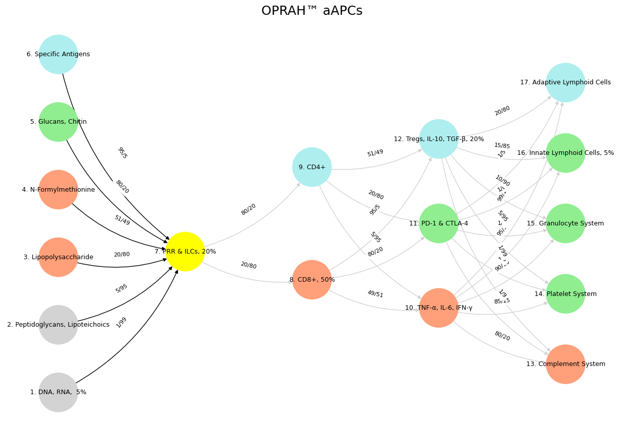
Fig. 24 Nvidia vs. Music. APIs between Nvidias CUDA (server) & their clients (yellowstone node: G1 & G2) are here replaced by the ear-drum (kuhura) & vestibular apparatus (space). The chief enterprise in music is listening and responding (N1, N2, N3) as well as coordination and syncronization with others too (N4 & N5). Whether its classical or improvisational and participatory (time), a massive and infinite combinatorial landscape is available for composer, maestro, performer, audience (rhythm). And who are we to say what exactly music optimizes (semantics)? The mammalian nervous system’s architecture can be mapped onto a neural network and the immune system, revealing a layered interplay of function. Layer 1’s six nodes, embodying cosmic laws and molecular inputs like DNA and antigens, align with the Red Queen Hypothesis, equating sensory and ecosystem via ligand-receptor complementarity. Layer 2, a yellow sentinel node (G1 & G2), parallels MHC and PRRs, relaying perception like cranial and dorsal ganglia. Layer 3’s two decision nodes—instinct (CD8+) versus tempered processes (CD4+)—mirror neural reflexes and modulation. Layer 4’s three equilibrium nodes—self (TNF-α), mutual (PD-1), and other (Tregs)—reflect sympathetic, parasympathetic, and transactional balance. Layer 5’s five metrics (complement to lymphoid cells) optimize responses, akin to neural integration of experience and environment. This mapping highlights a unified biological logic across systems, from static foundations to adaptive outcomes.