Traditional

The five sequences—Nihilism through Integration, Lens, Fragmented to United, Hate to Trust, and Cacophony to Symphony—offer a lens to explore bypassing the Institutional Review Board (IRB) process, often seen as an inefficient bottleneck, within the clinical research ecosystem. This ecosystem, involving students, professors, care providers, patients, analysts, academic departments, administrators, and federal employees with NHANES access, powers a web app for living donor nephrectomy decisions, generating Kaplan-Meier curves from harmonized donor and NHANES data. By leveraging clear, established workflows—like GitHub collaborations with public and private repositories, where identified and de-identified data are explicitly labeled—these sequences suggest how IRB inefficiencies might be sidestepped, streamlining data integration while preserving ethical integrity.

Fig. 37 I’d advise you to consider your position carefully (layer 3 fork in the road), perhaps adopting a more flexible posture (layer 4 dynamic capabilities realized), while keeping your ear to the ground (layer 2 yellow node), covering your retreat (layer 5 Athena’s shield, helmet, and horse), and watching your rear (layer 1 ecosystem and perspective).

The first sequence, Nihilism to Integration, reimagines bypassing IRB as a path from stagnation to efficiency. Nihilism, a failure to integrate, mirrors the IRB’s drag: delays in approving donor data sharing stall analysts’ Cox regression outputs, leaving NHANES controls and patient inputs unmerged. Deconstruction critiques this—why wait when GitHub workflows, with public repos for de-identified NHANES baselines and private ones for identified donor stats, clarify data use? Perspective sees the ecosystem’s potential: labeled datasets (e.g., “de-id_age” vs. “id_patient”) enable seamless collaboration. Awareness drives adoption of pre-set protocols—standardized .csv structures on GitHub—while Reconstruction builds the app’s back end without IRB lag. Integration delivers the Lens, its 95% CIs flowing from harmonized, workflow-tracked data. Here, bypassing IRB hinges on transparency: clear labels and established platforms replace oversight with accountability.

“Lens,” the second sequence, is the web app—a proof-of-concept for IRB-free integration. Hosted on GitHub Pages, it pulls from public de-identified NHANES functions and private donor .csv files, labeled explicitly (e.g., “public_cum_inc” vs. “private_beta_coeffs”). JavaScript and HTML fuse these via drop-down inputs, bypassing IRB by ensuring patients only see anonymized outputs—curves for perioperative mortality or ESRD risk—while analysts and professors collaborate in real time on GitHub. Sparse data (e.g., elderly donors) widens CIs, but pre-labeled workflows signal this upfront, sidestepping IRB’s slow consent reviews. The Lens thrives on this clarity: public-private delineation and versioned commits replace bureaucratic gatekeeping, showing how standardization within workflows can render IRB redundant.

Fragmented to United, the third sequence, reflects the unification enabled by bypassing IRB. Fragmentation festers under IRB delays—donor registries and NHANES remain siloed, skewing the app’s baseline vs. nephrectomy curves. With GitHub, public repos share harmonized, de-identified controls, while private ones house identified donor specifics, labeled for restricted access (e.g., “de-id_risk” vs. “id_event”). This clarity unites stakeholders: analysts merge data without waiting, care providers trust pre-vetted outputs, and patients see consistent risks. The challenge is ensuring labels hold—missteps (e.g., leaking identified data) invite scrutiny—but when executed, this workflow unites the ecosystem faster than IRB cycles, proving efficiency through structured transparency.

The fourth sequence, Hate to Trust, navigates the trust dynamics of bypassing IRB. “Hate” erupts as skepticism—patients fear unapproved data use, administrators dread liability, and federal employees resist sharing NHANES without oversight. “Negotiate” leverages workflows: public repos signal safety with de-identified data, private ones limit access to vetted collaborators (e.g., “private_donor_access:analyst1”), and labels like “IRB-exempt” justify the bypass. “Trust” emerges as the app delivers—curves align with reality, validated by GitHub’s audit trail, not IRB stamps. This shift reveals a trade-off: bypassing IRB demands robust self-regulation—clear labeling and access controls—to win stakeholder buy-in, replacing slow approvals with fast, transparent collaboration.

Cacophony to Symphony, the fifth sequence, harmonizes the chaos of bypassing IRB. “Cacophony” arises from unregulated data—unlabeled donor notes, NHANES noise, analysts’ unchecked tweaks—risking discord. “Outside” uses public GitHub repos to standardize de-identified NHANES inputs, while “Emotion” captures the tension: patients’ unease, professors’ ethics concerns. “Inside” refines this via private repos, where identified data (e.g., “id_periop_outcome”) is siloed yet harmonized with public baselines. “Symphony” sings as the app integrates these cleanly—curves reflect a unified truth, workflows prove compliance. This arc shows bypassing IRB amplifies efficiency when workflows orchestrate data with precision, turning potential anarchy into a streamlined chorus. Bypassing IRB, as seen here, leans on established GitHub workflows—public for de-identified, private for identified, all labeled—to outpace traditional oversight. The app, merging NHANES and donor data into actionable curves, proves this can work: efficiency soars when transparency and standardization replace delays. Beyond medicine—think tech firms or policy research—this scales wherever clear workflows can self-regulate, challenging IRB’s monopoly on ethics with a faster, equally accountable alternative. The risk? Human error in labeling or access. The reward? A nimble ecosystem, unbound by red tape, delivering insight at speed.

Show code cell source Hide code cell source

import numpy as np
import matplotlib.pyplot as plt
import networkx as nx

# Define the neural network layers
def define_layers():
    return {
        'Suis': ['DNA, RNA,  5%', 'Peptidoglycans, Lipoteichoics', 'Lipopolysaccharide', 'N-Formylmethionine', "Glucans, Chitin", 'Specific Antigens'],
        'Voir': ['PRR & ILCs, 20%'],  
        'Choisis': ['CD8+, 50%', 'CD4+'],  
        'Deviens': ['TNF-α, IL-6, IFN-γ', 'PD-1 & CTLA-4', 'Tregs, IL-10, TGF-β, 20%'],  
        "M'èléve": ['Complement System', 'Platelet System', 'Granulocyte System', 'Innate Lymphoid Cells, 5%', 'Adaptive Lymphoid Cells']  
    }

# Assign colors to nodes
def assign_colors():
    color_map = {
        'yellow': ['PRR & ILCs, 20%'],  
        'paleturquoise': ['Specific Antigens', 'CD4+', 'Tregs, IL-10, TGF-β, 20%', 'Adaptive Lymphoid Cells'],  
        'lightgreen': ["Glucans, Chitin", 'PD-1 & CTLA-4', 'Platelet System', 'Innate Lymphoid Cells, 5%', 'Granulocyte System'],  
        'lightsalmon': ['Lipopolysaccharide', 'N-Formylmethionine', 'CD8+, 50%', 'TNF-α, IL-6, IFN-γ', 'Complement System'],
    }
    return {node: color for color, nodes in color_map.items() for node in nodes}

# Define edge weights
def define_edges():
    return {
        ('DNA, RNA,  5%', 'PRR & ILCs, 20%'): '1/99',
        ('Peptidoglycans, Lipoteichoics', 'PRR & ILCs, 20%'): '5/95',
        ('Lipopolysaccharide', 'PRR & ILCs, 20%'): '20/80',
        ('N-Formylmethionine', 'PRR & ILCs, 20%'): '51/49',
        ("Glucans, Chitin", 'PRR & ILCs, 20%'): '80/20',
        ('Specific Antigens', 'PRR & ILCs, 20%'): '95/5',
        ('PRR & ILCs, 20%', 'CD8+, 50%'): '20/80',
        ('PRR & ILCs, 20%', 'CD4+'): '80/20',
        ('CD8+, 50%', 'TNF-α, IL-6, IFN-γ'): '49/51',
        ('CD8+, 50%', 'PD-1 & CTLA-4'): '80/20',
        ('CD8+, 50%', 'Tregs, IL-10, TGF-β, 20%'): '95/5',
        ('CD4+', 'TNF-α, IL-6, IFN-γ'): '5/95',
        ('CD4+', 'PD-1 & CTLA-4'): '20/80',
        ('CD4+', 'Tregs, IL-10, TGF-β, 20%'): '51/49',
        ('TNF-α, IL-6, IFN-γ', 'Complement System'): '80/20',
        ('TNF-α, IL-6, IFN-γ', 'Platelet System'): '85/15',
        ('TNF-α, IL-6, IFN-γ', 'Granulocyte System'): '90/10',
        ('TNF-α, IL-6, IFN-γ', 'Innate Lymphoid Cells, 5%'): '95/5',
        ('TNF-α, IL-6, IFN-γ', 'Adaptive Lymphoid Cells'): '99/1',
        ('PD-1 & CTLA-4', 'Complement System'): '1/9',
        ('PD-1 & CTLA-4', 'Platelet System'): '1/8',
        ('PD-1 & CTLA-4', 'Granulocyte System'): '1/7',
        ('PD-1 & CTLA-4', 'Innate Lymphoid Cells, 5%'): '1/6',
        ('PD-1 & CTLA-4', 'Adaptive Lymphoid Cells'): '1/5',
        ('Tregs, IL-10, TGF-β, 20%', 'Complement System'): '1/99',
        ('Tregs, IL-10, TGF-β, 20%', 'Platelet System'): '5/95',
        ('Tregs, IL-10, TGF-β, 20%', 'Granulocyte System'): '10/90',
        ('Tregs, IL-10, TGF-β, 20%', 'Innate Lymphoid Cells, 5%'): '15/85',
        ('Tregs, IL-10, TGF-β, 20%', 'Adaptive Lymphoid Cells'): '20/80'
    }

# Define edges to be highlighted in black
def define_black_edges():
    return {
        ('DNA, RNA,  5%', 'PRR & ILCs, 20%'): '1/99',
        ('Peptidoglycans, Lipoteichoics', 'PRR & ILCs, 20%'): '5/95',
        ('Lipopolysaccharide', 'PRR & ILCs, 20%'): '20/80',
        ('N-Formylmethionine', 'PRR & ILCs, 20%'): '51/49',
        ("Glucans, Chitin", 'PRR & ILCs, 20%'): '80/20',
        ('Specific Antigens', 'PRR & ILCs, 20%'): '95/5',
    }

# Calculate node positions
def calculate_positions(layer, x_offset):
    y_positions = np.linspace(-len(layer) / 2, len(layer) / 2, len(layer))
    return [(x_offset, y) for y in y_positions]

# Create and visualize the neural network graph
def visualize_nn():
    layers = define_layers()
    colors = assign_colors()
    edges = define_edges()
    black_edges = define_black_edges()
    
    G = nx.DiGraph()
    pos = {}
    node_colors = []
    
    # Create mapping from original node names to numbered labels
    mapping = {}
    counter = 1
    for layer in layers.values():
        for node in layer:
            mapping[node] = f"{counter}. {node}"
            counter += 1
            
    # Add nodes with new numbered labels and assign positions
    for i, (layer_name, nodes) in enumerate(layers.items()):
        positions = calculate_positions(nodes, x_offset=i * 2)
        for node, position in zip(nodes, positions):
            new_node = mapping[node]
            G.add_node(new_node, layer=layer_name)
            pos[new_node] = position
            node_colors.append(colors.get(node, 'lightgray'))
    
    # Add edges with updated node labels
    edge_colors = []
    for (source, target), weight in edges.items():
        if source in mapping and target in mapping:
            new_source = mapping[source]
            new_target = mapping[target]
            G.add_edge(new_source, new_target, weight=weight)
            edge_colors.append('black' if (source, target) in black_edges else 'lightgrey')
    
    # Draw the graph
    plt.figure(figsize=(12, 8))
    edges_labels = {(u, v): d["weight"] for u, v, d in G.edges(data=True)}
    
    nx.draw(
        G, pos, with_labels=True, node_color=node_colors, edge_color=edge_colors,
        node_size=3000, font_size=9, connectionstyle="arc3,rad=0.2"
    )
    nx.draw_networkx_edge_labels(G, pos, edge_labels=edges_labels, font_size=8)
    plt.title("OPRAH™ aAPCs", fontsize=18)
    plt.show()

# Run the visualization
visualize_nn()

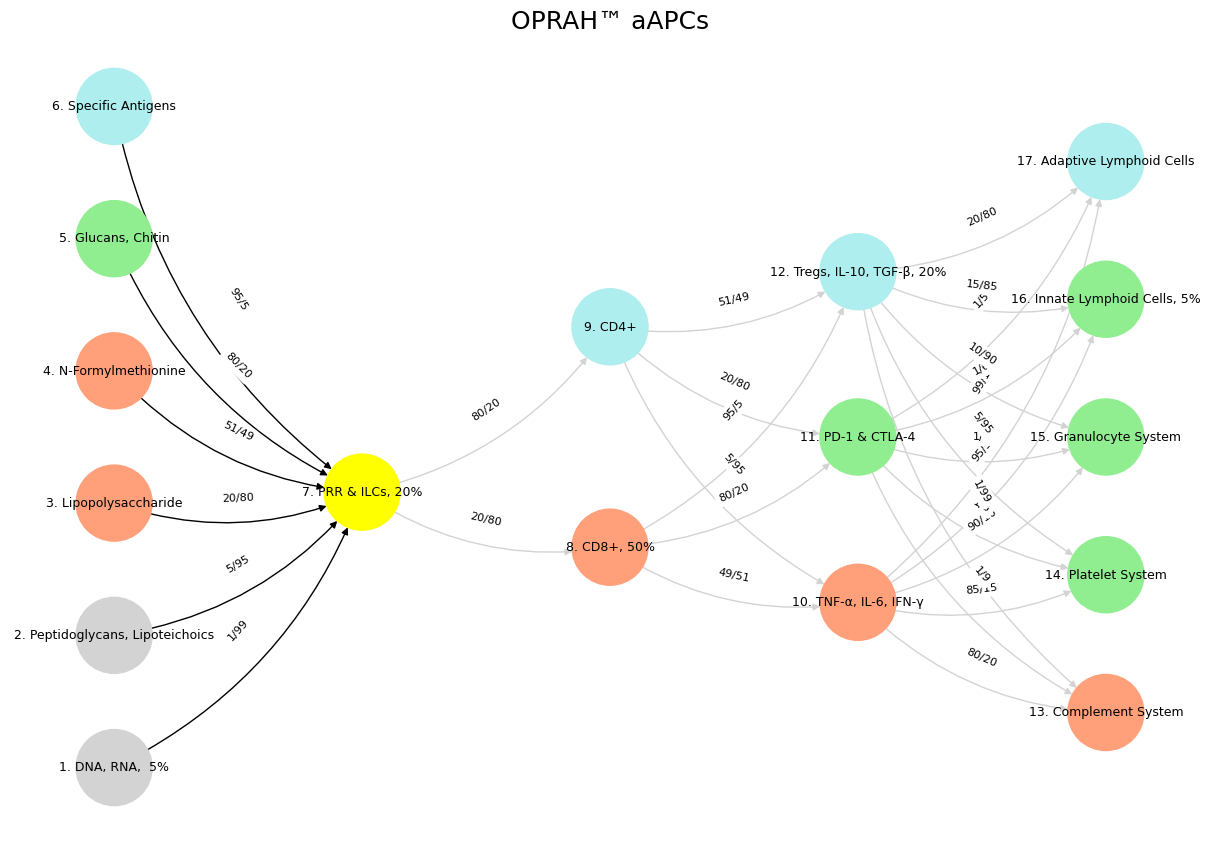
Fig. 38 While neural biology inspired neural networks in machine learning, the realization that scaling laws apply so beautifully to machine learning has led to a divergence in the process of generation of intelligence. Biology is constrained by the Red Queen, whereas mankind is quite open to destroying the Ecosystem-Cost function for the sake of generating the most powerful AI.