Veiled Resentment

The five sequences—Nihilism through Integration, Lens, Fragmented to United, Hate to Trust, and Cacophony to Symphony—offer a compelling lens to analyze data sharing within the clinical research ecosystem, as exemplified by a web app for living donor nephrectomy decisions. This ecosystem, populated by students, professors, care providers, patients, analysts, academic departments, administrators, and federal employees with NHANES access, hinges on the flow of data—donor registries, NHANES controls, Cox regression outputs—to generate Kaplan-Meier curves for outcomes like perioperative mortality or ESRD risk. Each sequence reveals how data sharing shapes this network, exposing barriers, negotiations, and the push toward integration that powers tools like the app.

Fig. 27 Uddin: a Kindred Spirit. Our gh-pages based ecosystem integration & navigation (EIN) framework is a competitive solution to a diagnosis we reached independently of Uddin. Source: Draft Complaint

The first sequence, Nihilism to Integration, frames data sharing as a journey from stagnation to synergy. Nihilism, a failure to integrate, emerges when data is hoarded: a professor guards IRB-approved donor data, an analyst’s .csv file with beta coefficients languishes on a private drive, or NHANES controls remain locked behind federal firewalls. Deconstruction dismantles these silos—imagine a student advocating for open GitHub repositories. Perspective dawns as stakeholders see the cost of isolation: unshared data limits the app’s accuracy. Awareness sparks a shift—analysts recognize NHANES could refine their variance-covariance matrix. Reconstruction drives collaborative action, merging donor and control datasets, and Integration births the app’s back end, hosted on GitHub Pages, where shared data fuels interactive curves. This arc underscores data sharing as the ecosystem’s lifeline, transforming fragmented knowledge into a unified resource.

“Lens,” the second sequence, is the web app itself—a QR-coded conduit for data sharing. Its JavaScript and HTML framework pulls from a .csv file, blending professors’ donor data, analysts’ Cox regression outputs, and federal NHANES baselines. Patients input demographics via drop-down menus, their data shaping real-time 95% CIs—wild for an 85-year-old donor due to sparse records. Analysts share model tweaks, administrators ensure IRB compliance, and care providers relay outcomes back into the system. The Lens thrives on this multidirectional flow: data moves from siloed sources to a public platform, enabling stakeholders to co-create a tool that balances precision and uncertainty. It reveals data sharing as a dynamic act, amplifying the ecosystem’s reach through accessibility and iteration.

Fragmented to United, the third sequence, reflects data sharing’s binary stakes. Fragmentation dominates when data sits apart—donor registries unlinked to NHANES, student analyses detached from clinical feedback. The app’s two curves (baseline vs. nephrectomy) demand unity: analysts must share regression coefficients, professors their datasets, and federal employees their controls to build a coherent picture. This process bridges gaps—patients see integrated risks, care providers align with research outputs. Yet, it’s fragile: incomplete sharing (e.g., missing elderly donor data) widens CIs, undermining trust. This sequence shows data sharing as the ecosystem’s glue, uniting disparate strands into a decision-making nexus, though gaps persist as a constant challenge.

The fourth sequence, Hate to Trust, maps the tensions and resolutions of data sharing. “Hate” flares as mistrust—patients doubt sparse data’s reliability, analysts resent professors withholding raw files, or administrators fear breaches in sharing NHANES extracts. “Negotiate” emerges as stakeholders bargain: a federal employee releases anonymized controls, a professor trades donor stats for co-authorship, a patient consents to data use for better curves. “Trust” solidifies when sharing pays off—the app’s outputs align with reality, validated by integrated datasets. This interplay highlights data sharing as a relational dance: friction over ownership or ethics yields to mutual benefit, with the Lens mediating by turning shared data into actionable insight.

Cacophony to Symphony, the fifth sequence, captures the noisy evolution of data sharing. “Cacophony” erupts from clashing data streams—unstandardized donor records, NHANES discrepancies, analysts’ competing models—creating chaos. “Outside” points to external sources like federal archives, their data flooding in unevenly. “Emotion” reflects stakeholders’ reactions: frustration at delays, hope in collaboration. “Inside” sees the app refine this mess—merging inputs into a base-case cumulative incidence function. “Symphony” arrives as shared data harmonizes: patients view polished curves, professors publish, administrators approve. This sequence portrays data sharing as a messy symphony, its discord resolved through iterative exchange, with the app as both conductor and score.

Data sharing, as seen here, is the ecosystem’s bloodstream—vital yet fraught. Silos (Nihilism) choke it; tools like the app (Lens) channel it; unity (United) depends on it; trust (Trust) sustains it; and coherence (Symphony) crowns it. Beyond nephrectomy, this applies to any data-driven system—tech firms pooling APIs, governments merging census stats—where sharing bridges isolation to empowerment. The app, born from a GitHub-shared script, proves data’s power lies not in hoarding but in flow, knitting stakeholders into a tapestry of informed choice.

Show code cell source Hide code cell source

import numpy as np
import matplotlib.pyplot as plt
import networkx as nx

# Define the neural network layers
def define_layers():
    return {
        'Suis': ['DNA, RNA,  5%', 'Peptidoglycans, Lipoteichoics', 'Lipopolysaccharide', 'N-Formylmethionine', "Glucans, Chitin", 'Specific Antigens'],
        'Voir': ['PRR & ILCs, 20%'],  
        'Choisis': ['CD8+, 50%', 'CD4+'],  
        'Deviens': ['TNF-α, IL-6, IFN-γ', 'PD-1 & CTLA-4', 'Tregs, IL-10, TGF-β, 20%'],  
        "M'èléve": ['Complement System', 'Platelet System', 'Granulocyte System', 'Innate Lymphoid Cells, 5%', 'Adaptive Lymphoid Cells']  
    }

# Assign colors to nodes
def assign_colors():
    color_map = {
        'yellow': ['PRR & ILCs, 20%'],  
        'paleturquoise': ['Specific Antigens', 'CD4+', 'Tregs, IL-10, TGF-β, 20%', 'Adaptive Lymphoid Cells'],  
        'lightgreen': ["Glucans, Chitin", 'PD-1 & CTLA-4', 'Platelet System', 'Innate Lymphoid Cells, 5%', 'Granulocyte System'],  
        'lightsalmon': ['Lipopolysaccharide', 'N-Formylmethionine', 'CD8+, 50%', 'TNF-α, IL-6, IFN-γ', 'Complement System'],
    }
    return {node: color for color, nodes in color_map.items() for node in nodes}

# Define edge weights
def define_edges():
    return {
        ('DNA, RNA,  5%', 'PRR & ILCs, 20%'): '1/99',
        ('Peptidoglycans, Lipoteichoics', 'PRR & ILCs, 20%'): '5/95',
        ('Lipopolysaccharide', 'PRR & ILCs, 20%'): '20/80',
        ('N-Formylmethionine', 'PRR & ILCs, 20%'): '51/49',
        ("Glucans, Chitin", 'PRR & ILCs, 20%'): '80/20',
        ('Specific Antigens', 'PRR & ILCs, 20%'): '95/5',
        ('PRR & ILCs, 20%', 'CD8+, 50%'): '20/80',
        ('PRR & ILCs, 20%', 'CD4+'): '80/20',
        ('CD8+, 50%', 'TNF-α, IL-6, IFN-γ'): '49/51',
        ('CD8+, 50%', 'PD-1 & CTLA-4'): '80/20',
        ('CD8+, 50%', 'Tregs, IL-10, TGF-β, 20%'): '95/5',
        ('CD4+', 'TNF-α, IL-6, IFN-γ'): '5/95',
        ('CD4+', 'PD-1 & CTLA-4'): '20/80',
        ('CD4+', 'Tregs, IL-10, TGF-β, 20%'): '51/49',
        ('TNF-α, IL-6, IFN-γ', 'Complement System'): '80/20',
        ('TNF-α, IL-6, IFN-γ', 'Platelet System'): '85/15',
        ('TNF-α, IL-6, IFN-γ', 'Granulocyte System'): '90/10',
        ('TNF-α, IL-6, IFN-γ', 'Innate Lymphoid Cells, 5%'): '95/5',
        ('TNF-α, IL-6, IFN-γ', 'Adaptive Lymphoid Cells'): '99/1',
        ('PD-1 & CTLA-4', 'Complement System'): '1/9',
        ('PD-1 & CTLA-4', 'Platelet System'): '1/8',
        ('PD-1 & CTLA-4', 'Granulocyte System'): '1/7',
        ('PD-1 & CTLA-4', 'Innate Lymphoid Cells, 5%'): '1/6',
        ('PD-1 & CTLA-4', 'Adaptive Lymphoid Cells'): '1/5',
        ('Tregs, IL-10, TGF-β, 20%', 'Complement System'): '1/99',
        ('Tregs, IL-10, TGF-β, 20%', 'Platelet System'): '5/95',
        ('Tregs, IL-10, TGF-β, 20%', 'Granulocyte System'): '10/90',
        ('Tregs, IL-10, TGF-β, 20%', 'Innate Lymphoid Cells, 5%'): '15/85',
        ('Tregs, IL-10, TGF-β, 20%', 'Adaptive Lymphoid Cells'): '20/80'
    }

# Define edges to be highlighted in black
def define_black_edges():
    return {
        ('Tregs, IL-10, TGF-β, 20%', 'Complement System'): '1/99',
        ('Tregs, IL-10, TGF-β, 20%', 'Platelet System'): '5/95',
        ('Tregs, IL-10, TGF-β, 20%', 'Granulocyte System'): '10/90',
        ('Tregs, IL-10, TGF-β, 20%', 'Innate Lymphoid Cells, 5%'): '15/85',
        ('Tregs, IL-10, TGF-β, 20%', 'Adaptive Lymphoid Cells'): '20/80'
    }

# Calculate node positions
def calculate_positions(layer, x_offset):
    y_positions = np.linspace(-len(layer) / 2, len(layer) / 2, len(layer))
    return [(x_offset, y) for y in y_positions]

# Create and visualize the neural network graph
def visualize_nn():
    layers = define_layers()
    colors = assign_colors()
    edges = define_edges()
    black_edges = define_black_edges()
    
    G = nx.DiGraph()
    pos = {}
    node_colors = []
    
    # Create mapping from original node names to numbered labels
    mapping = {}
    counter = 1
    for layer in layers.values():
        for node in layer:
            mapping[node] = f"{counter}. {node}"
            counter += 1
            
    # Add nodes with new numbered labels and assign positions
    for i, (layer_name, nodes) in enumerate(layers.items()):
        positions = calculate_positions(nodes, x_offset=i * 2)
        for node, position in zip(nodes, positions):
            new_node = mapping[node]
            G.add_node(new_node, layer=layer_name)
            pos[new_node] = position
            node_colors.append(colors.get(node, 'lightgray'))
    
    # Add edges with updated node labels
    edge_colors = []
    for (source, target), weight in edges.items():
        if source in mapping and target in mapping:
            new_source = mapping[source]
            new_target = mapping[target]
            G.add_edge(new_source, new_target, weight=weight)
            edge_colors.append('black' if (source, target) in black_edges else 'lightgrey')
    
    # Draw the graph
    plt.figure(figsize=(12, 8))
    edges_labels = {(u, v): d["weight"] for u, v, d in G.edges(data=True)}
    
    nx.draw(
        G, pos, with_labels=True, node_color=node_colors, edge_color=edge_colors,
        node_size=3000, font_size=9, connectionstyle="arc3,rad=0.2"
    )
    nx.draw_networkx_edge_labels(G, pos, edge_labels=edges_labels, font_size=8)
    plt.title("OPRAH™: Distributed Network", fontsize=18)
    plt.show()

# Run the visualization
visualize_nn()

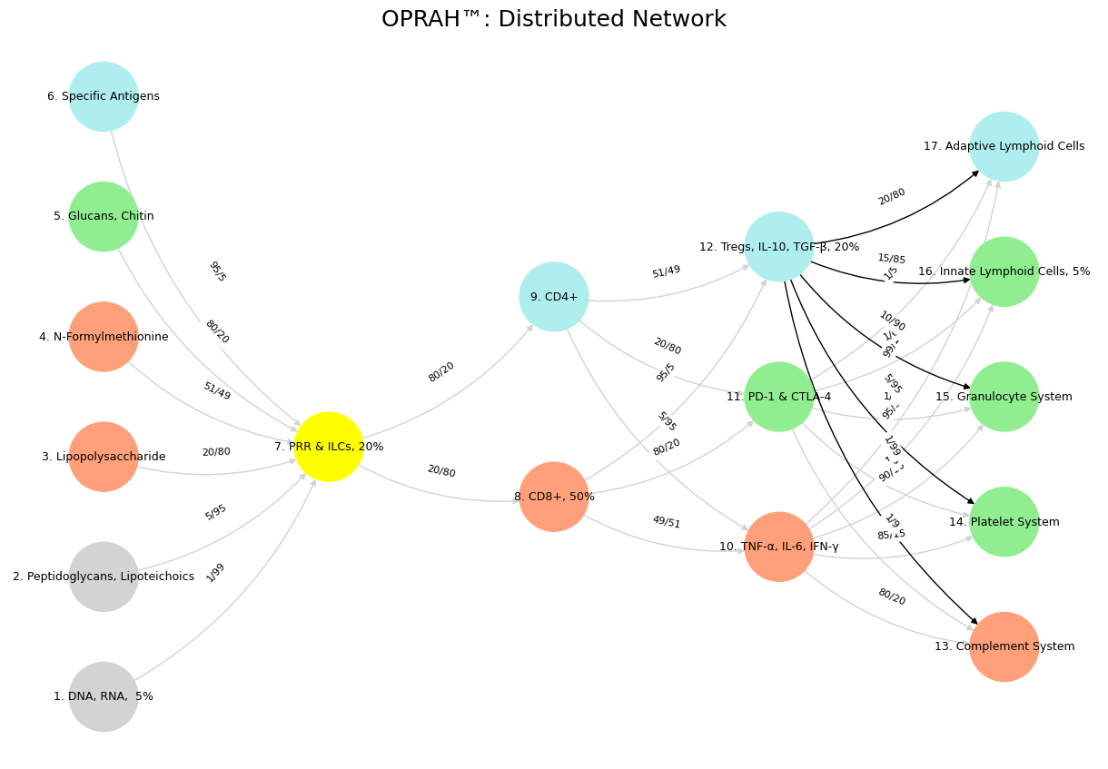
Fig. 28 Pericentral, Dorsal, Lateral, Medial, Cingulo-insular. These networks may be aligned with the five layers of our immunoneural network model to reveal convergence across completely unrelated biological and nonbiological systems. Importantly, the midcingulo-insular network (CIN), the most evolutionarily ancient and most conserved across mammal and nonmammalian animals, emerges as an integral hub in mediating dynamic interactions between other large-scale brain networks. As the output layer it can be viewed as the arbitrar of the “optimizaing funciton”, which turns out to be dynamic – unlike most human systems with fixed policies and credos.