Born to Etiquette

The five sequences—Nihilism through Integration, Lens, Fragmented to United, Hate to Trust, and Cacophony to Symphony—shed light on data harmonization methods within the clinical research ecosystem, as illustrated by a web app for living donor nephrectomy decisions. This ecosystem, encompassing students, professors, care providers, patients, analysts, academic departments, administrators, and federal employees with NHANES access, relies on harmonizing heterogeneous data—donor registries, NHANES controls, Cox regression outputs—to produce Kaplan-Meier curves for outcomes like perioperative mortality or ESRD risk. Each sequence reveals how harmonization methods bridge disparities, enabling the app to unify this complex network into a coherent tool for decision-making.

Fig. 34 He Does it Again. If we can send AIs to visit other planets and perhaps galaxies, surely aliens coud do the same and visit us. Thus UFOs are not that much of a stretch, especially in a nuclear world – aliens have recognized the “arrival” of another intelligence that has learned to harness the energy of the stars. We must overcome biological imperatives: status, tribe, etc. It’s clear that AI is one such approach. Matrix

The first sequence, Nihilism to Integration, portrays harmonization as a remedy for ecosystem breakdown. Nihilism, a failure to integrate, festers when donor data lists ages in ranges, NHANES uses raw counts, and analysts’ .csv files diverge in structure—unharmonized, they’re incompatible. Deconstruction employs profiling to dissect these differences, identifying variables like “mortality” coded differently across sources. Perspective emerges as stakeholders adopt semantic mapping, linking donor-specific risks to NHANES population norms. Awareness sparks the use of a common data model (e.g., OMOP), aligning fields like “sex” or “time-to-event.” Reconstruction applies transformation—converting disparate units (e.g., days to years)—and Integration delivers the app’s back end on GitHub Pages, where harmonized beta coefficients fuel consistent 95% CIs. Harmonization here turns chaos into cohesion, a painstaking climb from isolation to unity.

“Lens,” the second sequence, is the web app—a crucible for harmonization methods. Built with JavaScript and HTML, it merges NHANES cumulative incidence functions, donor stats, and patient inputs from drop-down menus into two curves. Record linkage harmonizes identifiers—matching “patient age” across datasets despite varied formats—while ontology alignment (e.g., SNOMED) unifies terms like “ESRD.” For sparse data (e.g., an 85-year-old donor), imputation borrows NHANES patterns to stabilize wide CIs. Analysts refine this via GitHub commits, administrators enforce IRB-aligned metadata, and care providers validate outputs. The Lens thrives when harmonization smooths these seams; without it, inputs like donor risks and NHANES baselines misalign, fracturing the app’s reliability and exposing harmonization’s precision as its backbone.

Fragmented to United, the third sequence, highlights harmonization’s role in resolving binary divides. Fragmentation persists when NHANES offers broad aggregates and donor data drills into specifics—unharmonized, they skew the app’s baseline vs. nephrectomy curves. Data fusion methods, like statistical matching, pair similar records (e.g., age-sex cohorts) across sources, while schema integration maps disparate fields into a shared structure. This unity empowers patients to compare risks reliably, but gaps—like missing elderly donor outcomes—test the limits: incomplete harmonization widens CIs, unsettling care providers. This sequence shows harmonization as a bridge, forging a single narrative from split datasets, though partial efforts leave cracks in the foundation.

The fourth sequence, Hate to Trust, frames harmonization as a trust catalyst amid stakeholder friction. “Hate” arises when unharmonized data sows doubt—patients question curves from mismatched metrics, analysts suspect professors’ hidden tweaks, federal employees withhold NHANES over format clashes. “Negotiate” leverages crosswalks—translating donor “event times” to NHANES scales—or consensus vocabularies (e.g., ICD-10), easing disputes. “Trust” blooms as harmonization proves its worth: the app’s outputs align when perioperative risks match across sources, reassuring all. This dynamic reveals harmonization’s human stakes: it demands agreement on standards, turning skepticism into reliance, with the Lens as the proving ground for shared, harmonized truth.

Cacophony to Symphony, the fifth sequence, captures harmonization’s triumph over data discord. “Cacophony” echoes in clashing inputs—donor free-text notes, NHANES statistical noise, analysts’ bespoke models—defying unity. “Outside” sees external NHANES data harmonized via ETL pipelines, extracting and transforming it to fit donor schemas. “Emotion” reflects the strain—students debug mismatches, patients face uncertain 30-year risks—but “Inside” applies normalization (e.g., standardizing risk scores), aligning inputs for the app’s base-case function. “Symphony” emerges as harmonized data sings: curves reflect a unified reality, stakeholders trust the result. This arc casts harmonization as a conductor, weaving noisy threads into harmony, though incomplete methods risk off-key notes.

These methods—profiling, mapping, fusion, transformation—anchor the ecosystem’s integration. For the nephrectomy app, they align NHANES to donor data, ensuring the Lens delivers clear curves despite sparse inputs (e.g., elderly donors). Beyond medicine, they scale to any fragmented system—tech syncing logs, policy blending surveys—where harmonization turns dissonance into dialogue. The app, fueled by a GitHub-hosted .csv, shows that without these techniques, data remains a cacophony; with them, it becomes a symphony of informed choice.

Show code cell source Hide code cell source

import numpy as np
import matplotlib.pyplot as plt
import networkx as nx

# Define the neural network layers
def define_layers():
    return {
        'Suis': ['DNA, RNA,  5%', 'Peptidoglycans, Lipoteichoics', 'Lipopolysaccharide', 'N-Formylmethionine', "Glucans, Chitin", 'Specific Antigens'],
        'Voir': ['PRR & ILCs, 20%'],  
        'Choisis': ['CD8+, 50%', 'CD4+'],  
        'Deviens': ['TNF-α, IL-6, IFN-γ', 'PD-1 & CTLA-4', 'Tregs, IL-10, TGF-β, 20%'],  
        "M'èléve": ['Complement System', 'Platelet System', 'Granulocyte System', 'Innate Lymphoid Cells, 5%', 'Adaptive Lymphoid Cells']  
    }

# Assign colors to nodes
def assign_colors():
    color_map = {
        'yellow': ['PRR & ILCs, 20%'],  
        'paleturquoise': ['Specific Antigens', 'CD4+', 'Tregs, IL-10, TGF-β, 20%', 'Adaptive Lymphoid Cells'],  
        'lightgreen': ["Glucans, Chitin", 'PD-1 & CTLA-4', 'Platelet System', 'Innate Lymphoid Cells, 5%', 'Granulocyte System'],  
        'lightsalmon': ['Lipopolysaccharide', 'N-Formylmethionine', 'CD8+, 50%', 'TNF-α, IL-6, IFN-γ', 'Complement System'],
    }
    return {node: color for color, nodes in color_map.items() for node in nodes}

# Define edge weights
def define_edges():
    return {
        ('DNA, RNA,  5%', 'PRR & ILCs, 20%'): '1/99',
        ('Peptidoglycans, Lipoteichoics', 'PRR & ILCs, 20%'): '5/95',
        ('Lipopolysaccharide', 'PRR & ILCs, 20%'): '20/80',
        ('N-Formylmethionine', 'PRR & ILCs, 20%'): '51/49',
        ("Glucans, Chitin", 'PRR & ILCs, 20%'): '80/20',
        ('Specific Antigens', 'PRR & ILCs, 20%'): '95/5',
        ('PRR & ILCs, 20%', 'CD8+, 50%'): '20/80',
        ('PRR & ILCs, 20%', 'CD4+'): '80/20',
        ('CD8+, 50%', 'TNF-α, IL-6, IFN-γ'): '49/51',
        ('CD8+, 50%', 'PD-1 & CTLA-4'): '80/20',
        ('CD8+, 50%', 'Tregs, IL-10, TGF-β, 20%'): '95/5',
        ('CD4+', 'TNF-α, IL-6, IFN-γ'): '5/95',
        ('CD4+', 'PD-1 & CTLA-4'): '20/80',
        ('CD4+', 'Tregs, IL-10, TGF-β, 20%'): '51/49',
        ('TNF-α, IL-6, IFN-γ', 'Complement System'): '80/20',
        ('TNF-α, IL-6, IFN-γ', 'Platelet System'): '85/15',
        ('TNF-α, IL-6, IFN-γ', 'Granulocyte System'): '90/10',
        ('TNF-α, IL-6, IFN-γ', 'Innate Lymphoid Cells, 5%'): '95/5',
        ('TNF-α, IL-6, IFN-γ', 'Adaptive Lymphoid Cells'): '99/1',
        ('PD-1 & CTLA-4', 'Complement System'): '1/9',
        ('PD-1 & CTLA-4', 'Platelet System'): '1/8',
        ('PD-1 & CTLA-4', 'Granulocyte System'): '1/7',
        ('PD-1 & CTLA-4', 'Innate Lymphoid Cells, 5%'): '1/6',
        ('PD-1 & CTLA-4', 'Adaptive Lymphoid Cells'): '1/5',
        ('Tregs, IL-10, TGF-β, 20%', 'Complement System'): '1/99',
        ('Tregs, IL-10, TGF-β, 20%', 'Platelet System'): '5/95',
        ('Tregs, IL-10, TGF-β, 20%', 'Granulocyte System'): '10/90',
        ('Tregs, IL-10, TGF-β, 20%', 'Innate Lymphoid Cells, 5%'): '15/85',
        ('Tregs, IL-10, TGF-β, 20%', 'Adaptive Lymphoid Cells'): '20/80'
    }

# Define edges to be highlighted in black
def define_black_edges():
    return {
        ('Tregs, IL-10, TGF-β, 20%', 'Complement System'): '1/99',
        ('Tregs, IL-10, TGF-β, 20%', 'Platelet System'): '5/95',
        ('Tregs, IL-10, TGF-β, 20%', 'Granulocyte System'): '10/90',
        ('Tregs, IL-10, TGF-β, 20%', 'Innate Lymphoid Cells, 5%'): '15/85',
        ('Tregs, IL-10, TGF-β, 20%', 'Adaptive Lymphoid Cells'): '20/80'
    }

# Calculate node positions
def calculate_positions(layer, x_offset):
    y_positions = np.linspace(-len(layer) / 2, len(layer) / 2, len(layer))
    return [(x_offset, y) for y in y_positions]

# Create and visualize the neural network graph
def visualize_nn():
    layers = define_layers()
    colors = assign_colors()
    edges = define_edges()
    black_edges = define_black_edges()
    
    G = nx.DiGraph()
    pos = {}
    node_colors = []
    
    # Create mapping from original node names to numbered labels
    mapping = {}
    counter = 1
    for layer in layers.values():
        for node in layer:
            mapping[node] = f"{counter}. {node}"
            counter += 1
            
    # Add nodes with new numbered labels and assign positions
    for i, (layer_name, nodes) in enumerate(layers.items()):
        positions = calculate_positions(nodes, x_offset=i * 2)
        for node, position in zip(nodes, positions):
            new_node = mapping[node]
            G.add_node(new_node, layer=layer_name)
            pos[new_node] = position
            node_colors.append(colors.get(node, 'lightgray'))
    
    # Add edges with updated node labels
    edge_colors = []
    for (source, target), weight in edges.items():
        if source in mapping and target in mapping:
            new_source = mapping[source]
            new_target = mapping[target]
            G.add_edge(new_source, new_target, weight=weight)
            edge_colors.append('black' if (source, target) in black_edges else 'lightgrey')
    
    # Draw the graph
    plt.figure(figsize=(12, 8))
    edges_labels = {(u, v): d["weight"] for u, v, d in G.edges(data=True)}
    
    nx.draw(
        G, pos, with_labels=True, node_color=node_colors, edge_color=edge_colors,
        node_size=3000, font_size=9, connectionstyle="arc3,rad=0.2"
    )
    nx.draw_networkx_edge_labels(G, pos, edge_labels=edges_labels, font_size=8)
    plt.title("OPRAH™: Distributed Network", fontsize=18)
    plt.show()

# Run the visualization
visualize_nn()

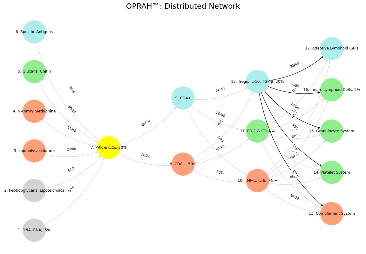
Fig. 35 Glenn Gould and Leonard Bernstein famously disagreed over the tempo and interpretation of Brahms’ First Piano Concerto during a 1962 New York Philharmonic concert, where Bernstein, conducting, publicly distanced himself from Gould’s significantly slower-paced interpretation before the performance began, expressing his disagreement with the unconventional approach while still allowing Gould to perform it as planned; this event is considered one of the most controversial moments in classical music history.