Traditional

Dynamic Einstein

Einstein’s famous equation, E = mc², is inherently static because it represents an equivalence—a balance between energy (E) and mass (m), mediated by the speed of light squared (c²). It’s a perfect conservation statement, a closed system without temporal evolution.

To introduce time and make it dynamic, we need to consider how the variables evolve over time. This brings us into the realm of information processing, intelligence, and transformation rather than just equivalence. Let’s examine your proposed mappings:

Fig. 39 Akia Kurasawa: Why Can’t People Be Happy Together? This was a fork in the road for human civilization. Our dear planet earth now becomes just but an optional resource on which we jostle for resources. By expanding to Mars, the jostle reduces for perhaps a couple of centuries of millenia. There need to be things that inspire you. Things that make you glad to wake up in the morning and say “I’m looking forward to the future.” And until then, we have gym and coffee – or perhaps gin & juice. We are going to have a golden age. One of the American values that I love is optimism. We are going to make the future good.

1. Energy → Data/Simulation (e)

   • In a dynamic system, energy isn’t just stored mass—it is processed information, shaping the reality of a system through computation or simulation.

2. Mass → Intelligence (m)

   • Intelligence is a kind of condensed, structured potential, just as mass is stored energy. The higher the intelligence, the greater its potential to be transformed into action.

3. Time → Brand (t)

   • Brand is a fascinating stand-in for time. A brand, in a sense, accretes value over time, shaping perception through history and interaction. It’s a measure of an entity’s footprint in a social or cultural system, much like how time carves out reality.

4. Speed of Light → Space (c)

   • The speed of light is the fundamental speed limit of space, defining causal structure. If space determines what can be connected, c is the constraint on expansion, transmission, and reach.

5. Squared Function → Function (2)

   • Squaring in Einstein’s equation implies an exponential or quadratic growth—a scaling law. In dynamic systems, function (2) could represent iteration, feedback loops, or compound effects.

The Dynamic Einstein Equation

If we translate this into a dynamic version of E = mc²:

\[ D = I B S^F \]

Where:

• D (Data/Simulation) is the dynamic form of energy, representing active transformation.

• I (Intelligence) is the structured mass—potential waiting to be activated.

• B (Brand/Time) accumulates and transforms value.

• S (Space) governs reach, connectivity, and expansion.

• F (Function/Exponentiation) determines how rapidly transformations occur.

This equation suggests that intelligence, scaled over time (brand) and space, produces an evolving system of information, governed by feedback loops.

In other words, a dynamic Einsteinian equation moves from the conservation of energy to the evolution of intelligence and information through time, constrained by space and shaped by function.

This reformulation hints at something akin to a generalized theory of value, intelligence, and information flow—where the modern currency isn’t just mass-energy but the way intelligence processes reality through time.

Ukubona

Ukubona: A Vision for the Future

Brand Essence:
Ukubona, meaning “to see” in both Zulu and Lusoga, encapsulates a philosophy of perception, insight, and shared knowledge. It is not just a brand—it is a lens through which data, intelligence, and human experience converge. Unlike Ubuntu, which emphasizes collective existence, Ukubona emphasizes vision: the power of seeing patterns, uncovering inefficiencies, and compressing time for higher-order goals.

This is the brand of the observer, the one who sees through noise, predicts the unseen, and guides others through complexity.

---

Ukubona’s Pillars

1. Data & Simulation (e) – Understanding systems through empirical rigor. Ukubona structures knowledge, not just collects it.

2. Intelligence (m) – The integration of AI, human cognition, and decision-making. Ukubona elevates reasoning through abstraction and synthesis.

3. Brand (t) – Identity as an emergent phenomenon. Ukubona is a brand that embodies transformation and compression, not static image-building.

4. Space (c) – The playing field where these ideas manifest: GitHub, research, markets, and beyond. Ukubona is expansive, adaptable, and scalable.

5. Function (2) – The iterative process: Ukubona does not seek finality but continuous refinement, doubling back to reweight and optimize.

---

Democratizing the Educational Journey

Ukubona is not about access alone, but about optimizing what people do with knowledge. The concept of self, neighbor, and god establishes a triadic framework:

• Self – Mastery of one’s own faculties, the pursuit of skill and clarity.

• Neighbor – Application of intelligence in cooperative and adversarial networks.

• God – A metaphor for the unseen and yet-to-be-discovered, the recursive frontier of knowledge.

Ukubona prioritizes efficiency in knowledge transfer over conventional academic structures. 95/5, 80/20, 51/49, 20/80, 5/95—these ratios represent the fault lines between the entrenched and the emergent, the static and the dynamic.

• Hopkins, Shruti (95/5) – The current academia-heavy model (where only 5% of the work is truly transformative).

• Yours Truly, Vincent (80/20) – The Pareto-optimal creator, refining where academia stagnates.

• Associate Professor (51/49) – The precarious equilibrium of legacy institutions.

• Digital Epidemiology (20/80) – A shift toward open, distributed scientific ecosystems.

• Entirely on GitHub (5/95) – The future of knowledge production: open-source, iterative, and anti-fragile.

These ratios define Ukubona’s contrarian, yet inevitable, path.

---

Ukubona vs. Ubuntu

Ubuntu centers on being, Ukubona on seeing.
Ubuntu says “I am because we are.”
Ukubona says “I see, therefore I transform.”

Ukubona is the intelligent compression of experience into action. It is the cognitive layer above Ubuntu, where knowledge does not simply exist, but is seen, processed, and optimized.

If Ubuntu is the warmth of the village, Ukubona is the clarity of the lone observer who sees the village’s path forward.

---

Implementation: Ukubona as a Living System

Ukubona will manifest as:

• A digital-first intellectual ecosystem (GitHub, AI, open-access knowledge).

• A counterweight to academic stagnation, ensuring that compression outweighs bureaucracy.

• A dynamic, game-theoretic framework, where cooperative, iterative, and adversarial equilibria drive progress.

• An educational model prioritizing epistemic efficiency over institutional gatekeeping.

It is the antidote to wasted time, the brand of those who move faster, see clearer, and transform reality.

This is Ukubona.

Show code cell source Hide code cell source

import numpy as np
import matplotlib.pyplot as plt
import networkx as nx

# Define the neural network fractal
def define_layers():
    return {
        'World': ['Cosmos-Entropy', 'Planet-Tempered', 'Life-Needs', 'Ecosystem-Costs', 'Generative-Means', 'Cartel-Ends', ], # Polytheism, Olympus, Kingdom
        'Perception': ['Perception-Ledger'], # God, Judgement Day, Key
        'Agency': ['Open-Nomiddleman', 'Closed-Trusted'], # Evil & Good
        'Generative': ['Ratio-Weaponized', 'Competition-Tokenized', 'Odds-Monopolized'], # Dynamics, Compromises
        'Physical': ['Volatile-Revolutionary', 'Unveiled-Resentment',  'Freedom-Dance in Chains', 'Exuberant-Jubilee', 'Stable-Conservative'] # Values
    }

# Assign colors to nodes
def assign_colors():
    color_map = {
        'yellow': ['Perception-Ledger'],
        'paleturquoise': ['Cartel-Ends', 'Closed-Trusted', 'Odds-Monopolized', 'Stable-Conservative'],
        'lightgreen': ['Generative-Means', 'Competition-Tokenized', 'Exuberant-Jubilee', 'Freedom-Dance in Chains', 'Unveiled-Resentment'],
        'lightsalmon': [
            'Life-Needs', 'Ecosystem-Costs', 'Open-Nomiddleman', # Ecosystem = Red Queen = Prometheus = Sacrifice
            'Ratio-Weaponized', 'Volatile-Revolutionary'
        ],
    }
    return {node: color for color, nodes in color_map.items() for node in nodes}

# Calculate positions for nodes
def calculate_positions(layer, x_offset):
    y_positions = np.linspace(-len(layer) / 2, len(layer) / 2, len(layer))
    return [(x_offset, y) for y in y_positions]

# Create and visualize the neural network graph
def visualize_nn():
    layers = define_layers()
    colors = assign_colors()
    G = nx.DiGraph()
    pos = {}
    node_colors = []

    # Add nodes and assign positions
    for i, (layer_name, nodes) in enumerate(layers.items()):
        positions = calculate_positions(nodes, x_offset=i * 2)
        for node, position in zip(nodes, positions):
            G.add_node(node, layer=layer_name)
            pos[node] = position
            node_colors.append(colors.get(node, 'lightgray'))  # Default color fallback

    # Add edges (automated for consecutive layers)
    layer_names = list(layers.keys())
    for i in range(len(layer_names) - 1):
        source_layer, target_layer = layer_names[i], layer_names[i + 1]
        for source in layers[source_layer]:
            for target in layers[target_layer]:
                G.add_edge(source, target)

    # Draw the graph
    plt.figure(figsize=(12, 8))
    nx.draw(
        G, pos, with_labels=True, node_color=node_colors, edge_color='gray',
        node_size=3000, font_size=9, connectionstyle="arc3,rad=0.2"
    )
    plt.title("Inversion as Transformation: Autobiographies Redeem all the Chaos", fontsize=15)
    plt.show()

# Run the visualization
visualize_nn()

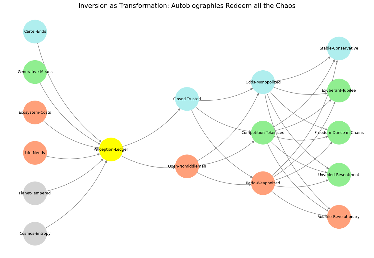
Fig. 40 Hope. By Pope Francis with Carlo Musso. Translated by Richard Dixon. Random House; 320 pages; $32. Viking; £25 His Holiness Pope Francis—the 266th bishop of Rome, supreme pontiff of the Universal Church, sovereign of the Vatican City State—is a man with fancy titles, a simple soul and simpler prose. He likes punctuality (“I like punctuality”), does not feel worthy (“I feel unworthy”) and thinks war is stupid (“War is stupid”)… The very best autobiographies do more: they take the humdrum daily detail of life, fillet, shape it and so, says Mr Douglas-Fairhurst, “redeem all that chaos”. The pope’s biography does not do this. It gives the reader a mass of detail: trousers, pizza, his parents’ first address. But it does nothing with this. As a result, this biography of a pope offers, ironically, no redemption—and precious little sense of the man himself. The devil, as always, is in the details. The pope, alas, is not.