Transvaluation

Combinatorial Spaces and Optimization Across Music, Survival Analysis, and Finance

The structure of equal temperament tuning, Cox proportional hazards regression, and option pricing models in finance reveals a striking unity across seemingly disparate domains. At their core, each system constructs a vast combinatorial space out of a fundamental unit—A440 in music, a baseline hazard in survival analysis, and a present value in finance—by applying exponential transformations. These transformations allow for infinite variation while preserving a parametric skeleton that makes predictions, expectations, and optimizations feasible. Yet, in each case, something is sacrificed: the pure harmonic series in music, the granularity of individual survival trajectories in epidemiology, and the full complexity of market behavior in finance. The sacrifice, in exchange for tractability and generalization, can lead to profound insights or catastrophic miscalculations, particularly when tail risks are underestimated. The question, then, is what exactly each of these fields is optimizing, and what data is required to generate intelligence from these optimization strategies.

Fig. 24 What Exactly is Identity. A node may represent goats (in general) and another sheep (in general). But the identity of any specific animal (not its species) is a network. For this reason we might have a “black sheep”, distinct in certain ways – perhaps more like a goat than other sheep. But that’s all dull stuff. Mistaken identity is often the fuel of comedy, usually when the adversarial is mistaken for the cooperative or even the transactional.

Music: The Optimization of Cadence

In music, the exponential structure of equal temperament (where each semitone is tuned as \( f_n = 440 \times 2^{n/12} \)) enables a vast combinatorial space of harmonic possibilities. The optimization problem in music is fundamentally one of expectation: the listener is guided through cycles of tension and resolution, with the cadence serving as the key point of satisfaction or frustration. The cycle of fifths, voice leading, chromatic modulations, and non-diatonic insertions all function as transformations that alter the expectation of resolution. The underlying intelligence in this optimization process is historical and cultural—the “data” comes from centuries of musical traditions, stylistic innovations, and the evolved neural responses of human cognition to harmonic progression. Just as certain paths in Cox regression are more likely given the survival curves of past populations, certain chord progressions carry emotional weight based on their historical and cultural frequency.

Yet, the equal temperament tuning system itself is a compromise, sacrificing the purity of harmonic overtones to enable modulation across all keys. The harmonic series—nature’s own tuning system—produces irrational frequency ratios that do not fit neatly into a system of 12 equal steps. In sacrificing just intonation, we gain an expandable, infinite harmonic space, but at the cost of an ever-present, almost imperceptible dissonance. This is the fundamental trade-off of parametric models: smooth generalization at the cost of localized precision.

Survival Analysis: The Optimization of Relative Risk

Cox proportional hazards regression follows a structurally similar mathematical form, where the probability of survival at a given time \( t \) is conditioned on a baseline hazard function \( h_0(t) \) multiplied by an exponential term:

\[ h(t) = h_0(t) \times e^{\beta X} \]

Here, the optimization problem is one of risk stratification—determining the probability that an individual with a given set of covariates \( X \) will experience an event (such as death, disease progression, or recovery) relative to a baseline group. This baseline group serves the same role as A440 in music: it is a reference point from which variations emerge. The exponentiated term, akin to the 12th-root-of-2 structure in equal temperament, allows for multiplicative scaling across different risk profiles.

The intelligence in survival analysis comes from epidemiological data, often extracted from national databases, electronic health records, or clinical trials. Unlike music, where the data emerges organically from creative evolution, survival analysis depends on structured, carefully collected data with well-defined endpoints. However, like equal temperament, Cox regression simplifies a more complex reality: it assumes proportional hazards, meaning the effect of a given risk factor remains constant over time. This is often not the case in real-world survival data, just as equal temperament is not the “natural” tuning system of harmonic series. When the assumption breaks down—when risk factors interact in non-linear or time-varying ways—the parametric model can mislead, sacrificing accuracy for mathematical tractability.

Finance: The Optimization of Expected Value in Option Pricing

In finance, the Black-Scholes model for European options follows a similar structural transformation, where the price of an option is given by:

\[ C = S_0 N(d_1) - Ke^{-rT} N(d_2) \]

Here, \( S_0 \) represents the current asset price (analogous to the baseline hazard or A440), while the exponential discounting term \( e^{-rT} \) mirrors the decay structure seen in Cox regression. The optimization problem is one of expectation: given an underlying asset and a time to maturity \( T \), what is the fair price of an option today? The combinatorial space is vast, allowing for hedging strategies, arbitrage opportunities, and derivatives of derivatives that layer exponentially.

The intelligence in financial modeling comes from market data—historical volatility, interest rates, and asset price movements. But, just as in equal temperament and survival analysis, the parametric form imposes a cost: it assumes log-normality in returns and smooth volatility dynamics, which, as history has shown, do not hold in extreme events. The financial crisis of 2008 was, in part, a failure of this parametric assumption. The tails of the distribution—akin to the enharmonic dissonances in music or the time-varying effects in Cox regression—were underestimated, leading to systemic collapse. The same elegant structure that makes financial engineering possible also makes it precarious when its assumptions are stretched beyond their intended domain.

Convergence and Divergence: The Sacrificial Altar of Parametric Models

In all three cases—music, survival analysis, and finance—the core structure consists of a baseline value modified by an exponential transformation. This mathematical consistency enables generalization and prediction but at the cost of local precision. Equal temperament sacrifices pure intervals for modularity, Cox regression sacrifices individual trajectories for proportionality, and Black-Scholes sacrifices tail risk for tractability. These sacrifices are what allow each field to construct vast combinatorial spaces, but they also introduce blind spots that can lead to aesthetic compromises, medical mispredictions, or financial disasters.

If we ask what is ultimately being optimized, the answer varies: in music, it is the listener’s expectation and resolution of cadence; in survival analysis, it is the relative risk estimation across populations; in finance, it is the expected value of future payouts. But all three require structured, historical data—whether from musical traditions, clinical trials, or market trends—to generate meaningful intelligence. The irony is that while these models enable powerful generative structures, they remain vulnerable to their own assumptions. When these assumptions fail, the sacrifices made at the altar of mathematical elegance come back to haunt us, often in the form of unexpected dissonances, survival paradoxes, or financial crises.

In the end, what we are truly optimizing is not just a function but an epistemology—the balance between abstraction and fidelity, between the infinite and the precise. The parametric structures that define our models are both our greatest tools and our most dangerous illusions.

Show code cell source Hide code cell source

import numpy as np
import matplotlib.pyplot as plt
import networkx as nx

# Define the neural network fractal
def define_layers():
    return {
        'World': ['Particles-Compression', 'Vibration-Particulate.Matter', 'Ear, Cerebellum-Georientation', 'Harmonic Series-Agency.Phonology', 'Space-Verb.Syntax', 'Time-Object.Meaning', ], # Resources, Strength
        'Perception': ['Rhythm, Pockets'], # Needs, Will
        'Agency': ['Open-Nomiddleman', 'Closed-Trusted'], # Costs, Cause
        'Generative': ['Ratio-Weaponized', 'Competition-Tokenized', 'Odds-Monopolized'], # Means, Ditto
        'Physical': ['Volatile-Revolutionary', 'Unveiled-Resentment',  'Freedom-Dance in Chains', 'Exuberant-Jubilee', 'Stable-Conservative'] # Ends, To Do
    }

# Assign colors to nodes
def assign_colors():
    color_map = {
        'yellow': ['Rhythm, Pockets'],
        'paleturquoise': ['Time-Object.Meaning', 'Closed-Trusted', 'Odds-Monopolized', 'Stable-Conservative'],
        'lightgreen': ['Space-Verb.Syntax', 'Competition-Tokenized', 'Exuberant-Jubilee', 'Freedom-Dance in Chains', 'Unveiled-Resentment'],
        'lightsalmon': [
            'Ear, Cerebellum-Georientation', 'Harmonic Series-Agency.Phonology', 'Open-Nomiddleman', 
            'Ratio-Weaponized', 'Volatile-Revolutionary'
        ],
    }
    return {node: color for color, nodes in color_map.items() for node in nodes}

# Calculate positions for nodes
def calculate_positions(layer, x_offset):
    y_positions = np.linspace(-len(layer) / 2, len(layer) / 2, len(layer))
    return [(x_offset, y) for y in y_positions]

# Create and visualize the neural network graph
def visualize_nn():
    layers = define_layers()
    colors = assign_colors()
    G = nx.DiGraph()
    pos = {}
    node_colors = []

    # Add nodes and assign positions
    for i, (layer_name, nodes) in enumerate(layers.items()):
        positions = calculate_positions(nodes, x_offset=i * 2)
        for node, position in zip(nodes, positions):
            G.add_node(node, layer=layer_name)
            pos[node] = position
            node_colors.append(colors.get(node, 'lightgray'))  # Default color fallback

    # Add edges (automated for consecutive layers)
    layer_names = list(layers.keys())
    for i in range(len(layer_names) - 1):
        source_layer, target_layer = layer_names[i], layer_names[i + 1]
        for source in layers[source_layer]:
            for target in layers[target_layer]:
                G.add_edge(source, target)

    # Draw the graph
    plt.figure(figsize=(12, 8))
    nx.draw(
        G, pos, with_labels=True, node_color=node_colors, edge_color='gray',
        node_size=3000, font_size=8, connectionstyle="arc3,rad=0.2"
    )
    plt.title("Music", fontsize=13)
    plt.show()

# Run the visualization
visualize_nn()

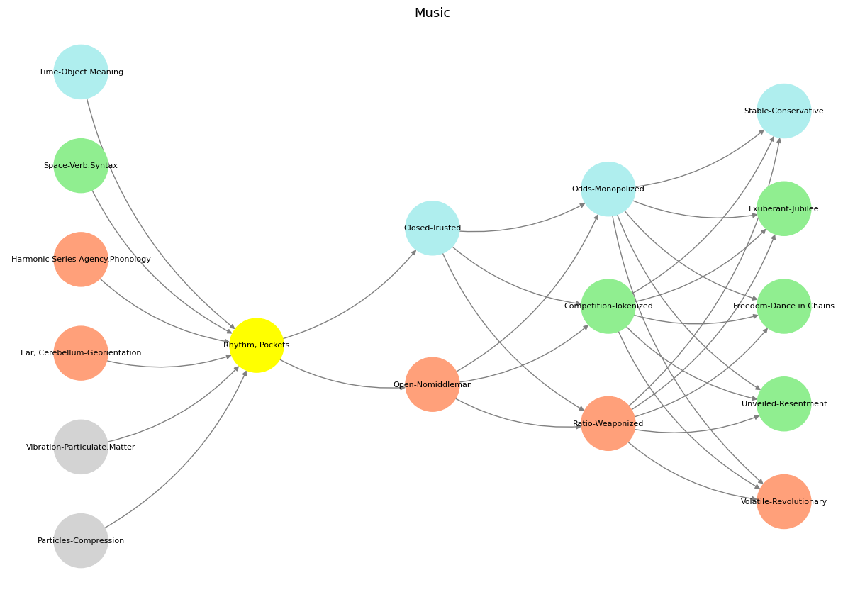
Fig. 25 Nvidia vs. Music. APIs between Nvidias CUDA & their clients (yellowstone node: G1 & G2) are here replaced by the ear-drum & vestibular apparatus. The chief enterprise in music is listening and responding (N1, N2, N3) as well as coordination and syncronization with others too (N4 & N5). Whether its classical or improvisational and participatory, a massive and infinite combinatorial landscape is available for composer, maestro, performer, audience. And who are we to say what exactly music optimizes?