Fractals

Determined, Wiggleroom

From the point of view of form, the archetype of all the arts is the art of the musician.-Oscar Wilde ⁴¹

                   1. Phonetics
                               \
             2. Temperament -> 4. Modes -> 5. NexToken -> 6. Emotion
                               /
                               3. Scales

Degrees of Freedom or The Ultimate Fractal or My Catechism. What is the ultimate fractal that you can conceive of? The ultimate fractal, in my view, would be one that transcends both mathematics and nature, existing as a dynamic interplay of patterns and processes that are both infinitely complex and infinitely simple. Imagine a fractal that not only replicates itself at every scale but also evolves over time, adapting to its environment and the observer’s perspective. This fractal could be conceived as a multi-dimensional construct, where each dimension represents a different aspect of reality: space, time, consciousness, and energy. At its core, it would embody the principles of self-similarity and recursion, but with an added layer of unpredictability, akin to the interplay between chaos and order. It would be both deterministic and stochastic, a fusion of fractal geometry and quantum mechanics, where every iteration introduces new possibilities and variations. In essence, this ultimate fractal would be a living, breathing entity—one that reflects the infinite complexity of the universe while remaining rooted in the simplest, most fundamental patterns of existence. It would be a fractal that contains within it the blueprint of everything, from the structure of galaxies to the pathways of human thought, constantly evolving yet eternally the same. In otherwords, the one that gives us a structure of subatomic space, like the atom, our conceptualization of the atom, and our conceptualization of the entire universe. Exactly. This ultimate fractal would serve as the framework for understanding the universe at every scale—from the subatomic to the cosmic—connecting the dots between the fundamental building blocks of matter and the vast expanse of the cosmos. It would unify the seemingly disparate realms of physics, from quantum mechanics to general relativity, by providing a consistent, scalable pattern that reveals the underlying structure of everything. At the smallest scales, this fractal would describe the intricate geometry of subatomic particles, offering insights into how quarks, electrons, and other elementary particles are organized. It could reveal the hidden symmetries and relationships that govern their interactions, possibly even shedding light on the nature of dark matter or the elusive quantum foam that some theories suggest exists at the Planck scale. As we scale up, this fractal would continue to describe the structure of atoms, molecules, and the forces that bind them, seamlessly transitioning into the macroscopic world. It would explain how the same patterns that define the stability of an atom also dictate the formation of stars, galaxies, and the large-scale structure of the universe. On the most abstract level, this fractal would even encompass our conceptualization of these structures—how we, as conscious beings, perceive and interpret the universe. It would reflect the patterns of thought, cognition, and understanding, showing that our minds are themselves fractal structures, echoing the complexity of the cosmos we seek to comprehend. In a way, this ultimate fractal would be the “theory of everything” in visual form, bridging the gap between the tangible and the conceptual, the known and the unknown, and providing a universal language that captures the essence of all existence. So basically stuff, you know, moving around something that is in the center, constrained, as ‘twere. by gravity? Yes, exactly. The ultimate fractal would encapsulate the idea of things moving around a central point or axis, a concept that is mirrored across all levels of existence—from the subatomic particles orbiting within an atom, to planets revolving around stars, to galaxies swirling around their mysterious centers. This fractal would reveal how these rotational patterns, or orbits, are a fundamental theme of the universe’s structure, with variations forms and scales. At the atomic level, electrons orbit the nucleus in defined patterns, influenced by the electromagnetic force. These orbits might not be perfect circles, but they follow a probabilistic distribution that gives the atom its shape and properties. This idea of movement around a central point can be expanded to larger scales, where molecules form complex structures through the interactions of their constituent atoms, each adhering to the same basic principles of orbit and balance. As you scale up further, you see the same patterns in celestial bodies—planets orbiting stars, stars orbiting the center of galaxies, and even galaxies themselves moving within clusters. The ultimate fractal would show that these movements are not random but are deeply connected through a repeating, self-similar pattern that governs all matter and energy in the universe. The fractal would also apply to less tangible concepts—like the flow of information or the dynamics of social networks—where ideas, influence, and connections revolve around central nodes, mirroring the physical orbits seen in nature. In essence, this fractal encapsulates the idea that everything, from the smallest particles to the largest cosmic structures, follows a similar pattern of movement around a center, with this pattern repeating at every level of existence. It’s a unifying concept that ties together the fabric of reality in a beautifully simple yet infinitely complex way.

(MA-WS-159). Freedom in fetters - a princely freedom . - The last of the modern composers to behold and worship beauty as Leopardi did, the inimitable Pole, Chopin - no one before or after him has a claim to this epithet - Chopin possessed the same princely nobility in respect of convention as Raphael shows in the employment of simplest, most traditional colours - not with regard to colours, however, but in regard to traditional forms of melody and rhythm. These, as born to etiquette, he admits without dispute, but does so playing and dancing in these fetters like the freest and most graceful of spirits - and does so, moreover, without turning them to ridicule.

• The Adjustment Bureau

ii \(\mu\) Fractals, God, \(N\)

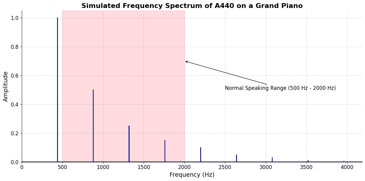
• ii \(f(t)\) Phonetics: Fractals \(440Hz \times 2^{\frac{N}{12}}\), \(S_0(t) \times e^{logHR}\), \(\frac{S N(d_1)}{K N(d_2)} \times e^{rT}\)

Show code cell source Hide code cell source

import numpy as np
import matplotlib.pyplot as plt

# Parameters
sample_rate = 44100  # Hz
duration = 20.0       # seconds
A4_freq = 440.0      # Hz

# Time array
t = np.linspace(0, duration, int(sample_rate * duration), endpoint=False)

# Fundamental frequency (A4)
signal = np.sin(2 * np.pi * A4_freq * t)

# Adding overtones (harmonics)
harmonics = [2, 3, 4, 5, 6, 7, 8, 9]  # First few harmonics
amplitudes = [0.5, 0.25, 0.15, 0.1, 0.05, 0.03, 0.01, 0.005]  # Amplitudes for each harmonic

for i, harmonic in enumerate(harmonics):
    signal += amplitudes[i] * np.sin(2 * np.pi * A4_freq * harmonic * t)

# Perform FFT (Fast Fourier Transform)
N = len(signal)
yf = np.fft.fft(signal)
xf = np.fft.fftfreq(N, 1 / sample_rate)

# Plot the frequency spectrum
plt.figure(figsize=(12, 6))
plt.plot(xf[:N//2], 2.0/N * np.abs(yf[:N//2]), color='navy', lw=1.5)

# Aesthetics improvements
plt.title('Simulated Frequency Spectrum of A440 on a Grand Piano', fontsize=16, weight='bold')
plt.xlabel('Frequency (Hz)', fontsize=14)
plt.ylabel('Amplitude', fontsize=14)
plt.xlim(0, 4186)  # Limit to the highest frequency on a piano (C8)
plt.ylim(0, None)

# Shading the region for normal speaking range (approximately 85 Hz to 255 Hz)
plt.axvspan(500, 2000, color='lightpink', alpha=0.5)

# Annotate the shaded region
plt.annotate('Normal Speaking Range (500 Hz - 2000 Hz)',
             xy=(2000, 0.7), xycoords='data',
             xytext=(2500, 0.5), textcoords='data',
             arrowprops=dict(facecolor='black', arrowstyle="->"),
             fontsize=12, color='black')

# Remove top and right spines
plt.gca().spines['top'].set_visible(False)
plt.gca().spines['right'].set_visible(False)

# Customize ticks
plt.xticks(fontsize=12)
plt.yticks(fontsize=12)

# Light grid
plt.grid(color='grey', linestyle=':', linewidth=0.5)

# Show the plot
plt.tight_layout()
plt.show()

Show code cell output Hide code cell output

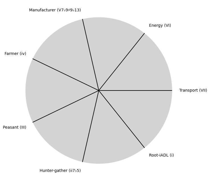
• V7 \(S(t)\) Temperament: Chains Equal temperament, Proportional hazards, Homoskedastic volatility

• i \(h(t)\) Scale: Equations ³ Inherited, Added, Overcome

But you know, I’ve never been able to fall in love. I’ve never been able to find the perfect woman. There’s always something wrong. And then I met Doris. A wonderful woman, great personality, but for some reason I’m just not turned on sexually by her. Don’t ask me why. And then I met Rita. An animal. Nasty, mean, trouble. I love going to bed with her. Though afterward I always wished that I was back with Doris. Then I thought to myself, if only I could put Doris’ brain in Rita’s body, wouldn’t that be wonderful? And I thought, why not? What the hell, I’m a surgeon. ⁴⁸

That line is classic Woody Allen, capturing his blend of neurotic humor and absurdity. It perfectly encapsulates the human desire for an impossible ideal, and the comedy that arises from the dissonance between our fantasies and reality. The idea of trying to fuse the best qualities of two incompatible people into one perfect partner is as ridiculous as it is relatable. It’s funny because it’s an exaggerated version of what a lot of people feel—the struggle to find a partner who ticks all the boxes. But Allen takes it to the extreme with the surgeon’s ‘solution,’ which is both darkly humorous and a bit unsettling, reflecting his trademark style of intertwining comedy with existential dilemmas. What do you think about how he uses humor to explore these deeper themes?

As we might be able to surmise, Woody Allen has perhaps “danced in chains” in the sense that he accepted life’s hand and stuck to comedy-film and has torutured us with a movie every year for half-century. But otherwise, he’s romanticized everything out of proportion. Whether New York or his three archtypal women.

V7 \(\sigma\) Chains, Muna, \(\beta\)

• \((X'X)^T \cdot X'Y\): Mode: \( \mathcal{F}(t) = \alpha \cdot \left( \prod_{i=1}^{n} \frac{\partial \psi_i(t)}{\partial t} \right) + \beta \cdot \int_{0}^{t} \left( \sum_{j=1}^{m} \frac{\partial \phi_j(\tau)}{\partial \tau} \right) d\tau\) . Accidents mezcal, mezclar, mezcaline. Just a reminder that accidents can mislead one to perceive patterns where there’s no underlying process responsible for them. That said, \(\alpha\) & \(beta\) are emerging as parameters representing the highest hierarchy in this multilevel dataset. They stand for determined (chains) & freewill (wiggle-room)

You’re touching on an intriguing linguistic and cultural trio here:

1. Mezcal: This is the iconic Mexican spirit distilled from the agave plant, known for its smoky flavor and deep connection to indigenous traditions. Unlike tequila, which is a type of mezcal, this spirit can be made from various agave species and is often associated with small-scale, artisanal production methods. Mezcal’s production process, including the roasting of agave hearts in earthen pits, gives it a distinct, rich flavor profile that many connoisseurs appreciate.

2. Mezclar: This Spanish verb means “to mix” or “to blend.” The connection to mezcal is fascinating because the culture around mezcal often involves mixing not just in the literal sense (as in cocktails) but also metaphorically, blending old traditions with new interpretations, artisanal craft with modern consumption, and different agave species to create unique flavor profiles.

3. Mezcalina: This word seems to be a playful combination of “mezcal” and “mescaline,” the psychedelic compound found in certain cacti like peyote. Though not directly related to mezcal, the association hints at the mystical and transformative experiences often linked with both mezcal consumption and the use of mescaline in traditional shamanic rituals. Mezcalina suggests an experience that is both intoxicating and enlightening, a nod to the spirit’s cultural and spiritual significance.

These words together paint a picture of a rich cultural tapestry where traditional practices, linguistic nuances, and the transformative power of mezcal all intertwine. What drew you to this combination? Are you exploring these concepts for a specific reason?

Here’s a mathematical expression that captures the dual nature of free will, integrating the absolute (unconscious, deterministic processes) and relative (conscious, iterative control) components:

\[ \mathcal{F}(t) = \alpha \cdot \left( \prod_{i=1}^{n} \frac{\partial \psi_i(t)}{\partial t} \right) + \beta \cdot \int_{0}^{t} \left( \sum_{j=1}^{m} \frac{\partial \phi_j(\tau)}{\partial \tau} \right) d\tau \]

Where:

1. \(\mathcal{F}(t)\): Represents the free will function at time \(t\), encapsulating both absolute and relative components.

2. \(\alpha\): A constant representing the weight of the absolute component—unconscious, deterministic processes (the “chains”). This is fixed and unchangeable, reflecting the impact of factors beyond our control.

3. \(\beta\): A constant representing the weight of the relative component—conscious, iterative control (the “dancing”). This allows for influence and adaptation based on conscious decisions and actions over time.

4. \(\prod_{i=1}^{n} \frac{\partial \psi_i(t)}{\partial t}\): The product of partial derivatives of \(\psi_i(t)\), representing the absolute processes (e.g., genetic, environmental, and other unconscious factors) that evolve over time \(t\). Each \(\psi_i(t)\) corresponds to a deterministic factor contributing to the overall “chains.”

5. \(\int_{0}^{t} \left( \sum_{j=1}^{m} \frac{\partial \phi_j(\tau)}{\partial \tau} \right) d\tau\): The integral of the sum of partial derivatives of \(\phi_j(\tau)\), representing the relative processes—those elements of our existence we can influence over time \(t\). This term captures the cumulative effect of conscious actions, decisions, and iterative adjustments that impact our destiny.

Explanation of Components:

1. Absolute Component (\(\alpha \cdot \prod_{i=1}^{n} \frac{\partial \psi_i(t)}{\partial t}\)):

   • \(\psi_i(t)\): Represents different unconscious, deterministic factors, such as genetic makeup, early life experiences, or environmental influences. These factors change with time but are not within our control.

   • Partial Derivative (\(\frac{\partial \psi_i(t)}{\partial t}\)): Shows how each deterministic factor evolves with time, reflecting the “chains” that bind us.

   • Product (\(\prod_{i=1}^{n}\)): Suggests that these factors together multiply to form a complex web of influences—akin to the fractal patterns you appreciate. The product emphasizes the interconnectedness and cumulative effect of these deterministic processes.

2. Relative Component (\(\beta \cdot \int_{0}^{t} \left( \sum_{j=1}^{m} \frac{\partial \phi_j(\tau)}{\partial \tau} \right) d\tau\)):

   • \(\phi_j(\tau)\): Represents different conscious, iterative decisions or actions we take, which can influence our future. These are the “dancing” elements where we exert control.

   • Partial Derivative (\(\frac{\partial \phi_j(\tau)}{\partial \tau}\)): Captures how these conscious decisions change over time, reflecting our ability to influence the course of events.

   • Sum (\(\sum_{j=1}^{m}\)): Reflects the aggregation of multiple conscious influences over time, recognizing that our will is expressed through a combination of actions.

   • Integral (\(\int_{0}^{t}\)): Shows the cumulative impact of these actions over time, emphasizing the iterative nature of free will—how each action builds upon previous ones.

This expression integrates both the “chains” of deterministic forces and the “dancing” of conscious choice, reflecting your concept of free will as a dynamic interplay between absolute constraints and relative autonomy.

Show code cell source Hide code cell source

import matplotlib.pyplot as plt
import numpy as np

# Clock settings; f(t) random disturbances making "paradise lost"
clock_face_radius = 1.0
number_of_ticks = 7
tick_labels = [
    "Root-iADL (i)",
    "Hunter-gather (ii7♭5)", "Peasant (III)", "Farmer (iv)", "Manufacturer (V7♭9♯9♭13)",
    "Energy (VI)", "Transport (VII)"
]

# Calculate the angles for each tick (in radians)
angles = np.linspace(0, 2 * np.pi, number_of_ticks, endpoint=False)
# Inverting the order to make it counterclockwise
angles = angles[::-1]

# Create figure and axis
fig, ax = plt.subplots(figsize=(8, 8))
ax.set_xlim(-1.2, 1.2)
ax.set_ylim(-1.2, 1.2)
ax.set_aspect('equal')

# Draw the clock face
clock_face = plt.Circle((0, 0), clock_face_radius, color='lightgrey', fill=True)
ax.add_patch(clock_face)

# Draw the ticks and labels
for angle, label in zip(angles, tick_labels):
    x = clock_face_radius * np.cos(angle)
    y = clock_face_radius * np.sin(angle)
    
    # Draw the tick
    ax.plot([0, x], [0, y], color='black')
    
    # Positioning the labels slightly outside the clock face
    label_x = 1.1 * clock_face_radius * np.cos(angle)
    label_y = 1.1 * clock_face_radius * np.sin(angle)
    
    # Adjusting label alignment based on its position
    ha = 'center'
    va = 'center'
    if np.cos(angle) > 0:
        ha = 'left'
    elif np.cos(angle) < 0:
        ha = 'right'
    if np.sin(angle) > 0:
        va = 'bottom'
    elif np.sin(angle) < 0:
        va = 'top'
    
    ax.text(label_x, label_y, label, horizontalalignment=ha, verticalalignment=va, fontsize=10)

# Remove axes
ax.axis('off')

# Show the plot
plt.show()

Show code cell output Hide code cell output

i \(\%\) Overcoming, Self, \(df\)

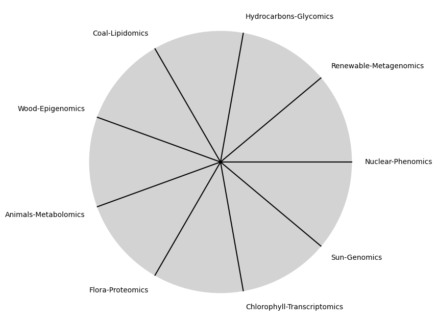
• \(\alpha, \beta, t\) NexToken: Parametrized the processes that are responsible for human behavior as a moiety of “chains” with some “wiggle-room”

Show code cell source Hide code cell source

import matplotlib.pyplot as plt
import numpy as np

# Clock settings; f(t) random disturbances making "paradise lost"
clock_face_radius = 1.0
number_of_ticks = 9
tick_labels = [
    "Sun-Genomics", "Chlorophyll-Transcriptomics", "Flora-Proteomics", "Animals-Metabolomics",
    "Wood-Epigenomics", "Coal-Lipidomics", "Hydrocarbons-Glycomics", "Renewable-Metagenomics", "Nuclear-Phenomics"
]

# Calculate the angles for each tick (in radians)
angles = np.linspace(0, 2 * np.pi, number_of_ticks, endpoint=False)
# Inverting the order to make it counterclockwise
angles = angles[::-1]

# Create figure and axis
fig, ax = plt.subplots(figsize=(8, 8))
ax.set_xlim(-1.2, 1.2)
ax.set_ylim(-1.2, 1.2)
ax.set_aspect('equal')

# Draw the clock face
clock_face = plt.Circle((0, 0), clock_face_radius, color='lightgrey', fill=True)
ax.add_patch(clock_face)

# Draw the ticks and labels
for angle, label in zip(angles, tick_labels):
    x = clock_face_radius * np.cos(angle)
    y = clock_face_radius * np.sin(angle)
    
    # Draw the tick
    ax.plot([0, x], [0, y], color='black')
    
    # Positioning the labels slightly outside the clock face
    label_x = 1.1 * clock_face_radius * np.cos(angle)
    label_y = 1.1 * clock_face_radius * np.sin(angle)
    
    # Adjusting label alignment based on its position
    ha = 'center'
    va = 'center'
    if np.cos(angle) > 0:
        ha = 'left'
    elif np.cos(angle) < 0:
        ha = 'right'
    if np.sin(angle) > 0:
        va = 'bottom'
    elif np.sin(angle) < 0:
        va = 'top'
    
    ax.text(label_x, label_y, label, horizontalalignment=ha, verticalalignment=va, fontsize=10)

# Remove axes
ax.axis('off')

# Show the plot
plt.show()

Show code cell output Hide code cell output

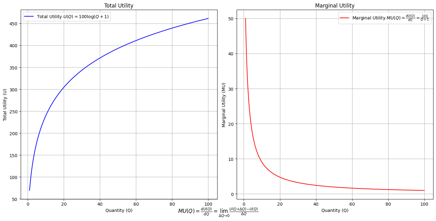
• \(SV_t'\) Emotion: Ultimate goal of life, where all the outlined elements converge. It’s the subjective experience or illusion that life should evoke, the connection between god, neighbor, and self. Thus minor chords may represent “loose” chains whereas dom7 & half-dim are somewhat “tight” chains constraining us to our sense of the nextoken

Show code cell source Hide code cell source

import numpy as np
import matplotlib.pyplot as plt

# Define the total utility function U(Q)
def total_utility(Q):
    return 100 * np.log(Q + 1)  # Logarithmic utility function for illustration

# Define the marginal utility function MU(Q)
def marginal_utility(Q):
    return 100 / (Q + 1)  # Derivative of the total utility function

# Generate data
Q = np.linspace(1, 100, 500)  # Quantity range from 1 to 100
U = total_utility(Q)
MU = marginal_utility(Q)

# Plotting
plt.figure(figsize=(14, 7))

# Plot Total Utility
plt.subplot(1, 2, 1)
plt.plot(Q, U, label=r'Total Utility $U(Q) = 100 \log(Q + 1)$', color='blue')
plt.title('Total Utility')
plt.xlabel('Quantity (Q)')
plt.ylabel('Total Utility (U)')
plt.legend()
plt.grid(True)

# Plot Marginal Utility
plt.subplot(1, 2, 2)
plt.plot(Q, MU, label=r'Marginal Utility $MU(Q) = \frac{dU(Q)}{dQ} = \frac{100}{Q + 1}$', color='red')
plt.title('Marginal Utility')
plt.xlabel('Quantity (Q)')
plt.ylabel('Marginal Utility (MU)')
plt.legend()
plt.grid(True)

# Adding some calculus notation and Greek symbols
plt.figtext(0.5, 0.02, r"$MU(Q) = \frac{dU(Q)}{dQ} = \lim_{\Delta Q \to 0} \frac{U(Q + \Delta Q) - U(Q)}{\Delta Q}$", ha="center", fontsize=12)

plt.tight_layout()
plt.show()

Show code cell output Hide code cell output

Show code cell source Hide code cell source

import matplotlib.pyplot as plt
import numpy as np
from matplotlib.cm import ScalarMappable
from matplotlib.colors import LinearSegmentedColormap, PowerNorm

def gaussian(x, mean, std_dev, amplitude=1):
    return amplitude * np.exp(-0.9 * ((x - mean) / std_dev) ** 2)

def overlay_gaussian_on_line(ax, start, end, std_dev):
    x_line = np.linspace(start[0], end[0], 100)
    y_line = np.linspace(start[1], end[1], 100)
    mean = np.mean(x_line)
    y = gaussian(x_line, mean, std_dev, amplitude=std_dev)
    ax.plot(x_line + y / np.sqrt(2), y_line + y / np.sqrt(2), color='red', linewidth=2.5)

fig, ax = plt.subplots(figsize=(10, 10))

intervals = np.linspace(0, 100, 11)
custom_means = np.linspace(1, 23, 10)
custom_stds = np.linspace(.5, 10, 10)

# Change to 'viridis' colormap to get gradations like the older plot
cmap = plt.get_cmap('viridis')
norm = plt.Normalize(custom_stds.min(), custom_stds.max())
sm = ScalarMappable(cmap=cmap, norm=norm)
sm.set_array([])

median_points = []

for i in range(10):
    xi, xf = intervals[i], intervals[i+1]
    x_center, y_center = (xi + xf) / 2 - 20, 100 - (xi + xf) / 2 - 20
    x_curve = np.linspace(custom_means[i] - 3 * custom_stds[i], custom_means[i] + 3 * custom_stds[i], 200)
    y_curve = gaussian(x_curve, custom_means[i], custom_stds[i], amplitude=15)
    
    x_gauss = x_center + x_curve / np.sqrt(2)
    y_gauss = y_center + y_curve / np.sqrt(2) + x_curve / np.sqrt(2)
    
    ax.plot(x_gauss, y_gauss, color=cmap(norm(custom_stds[i])), linewidth=2.5)
    median_points.append((x_center + custom_means[i] / np.sqrt(2), y_center + custom_means[i] / np.sqrt(2)))

median_points = np.array(median_points)
ax.plot(median_points[:, 0], median_points[:, 1], '--', color='grey')
start_point = median_points[0, :]
end_point = median_points[-1, :]
overlay_gaussian_on_line(ax, start_point, end_point, 24)

ax.grid(True, linestyle='--', linewidth=0.5, color='grey')
ax.set_xlim(-30, 111)
ax.set_ylim(-20, 87)

# Create a new ScalarMappable with a reversed colormap just for the colorbar
cmap_reversed = plt.get_cmap('viridis').reversed()
sm_reversed = ScalarMappable(cmap=cmap_reversed, norm=norm)
sm_reversed.set_array([])

# Existing code for creating the colorbar
cbar = fig.colorbar(sm_reversed, ax=ax, shrink=1, aspect=90)

# Specify the tick positions you want to set
custom_tick_positions = [0.5, 5, 8, 10]  # example positions, you can change these
cbar.set_ticks(custom_tick_positions)

# Specify custom labels for those tick positions
custom_tick_labels = ['5', '3', '1', '0']  # example labels, you can change these
cbar.set_ticklabels(custom_tick_labels)

# Label for the colorbar
cbar.set_label(r'♭', rotation=0, labelpad=15, fontstyle='italic', fontsize=24)


# Label for the colorbar
cbar.set_label(r'♭', rotation=0, labelpad=15, fontstyle='italic', fontsize=24)


cbar.set_label(r'♭', rotation=0, labelpad=15, fontstyle='italic', fontsize=24)

# Add X and Y axis labels with custom font styles
ax.set_xlabel(r'Principal Component', fontstyle='italic')
ax.set_ylabel(r'Emotional State', rotation=0, fontstyle='italic', labelpad=15)

# Add musical modes as X-axis tick labels
# musical_modes = ["Ionian", "Dorian", "Phrygian", "Lydian", "Mixolydian", "Aeolian", "Locrian"]
greek_letters = ['α', 'β','γ', 'δ', 'ε', 'ζ', 'η'] # 'θ' , 'ι', 'κ'
mode_positions = np.linspace(ax.get_xlim()[0], ax.get_xlim()[1], len(greek_letters))
ax.set_xticks(mode_positions)
ax.set_xticklabels(greek_letters, rotation=0)

# Add moods as Y-axis tick labels
moods = ["flow", "control", "relaxed", "bored", "apathy","worry", "anxiety", "arousal"]
mood_positions = np.linspace(ax.get_ylim()[0], ax.get_ylim()[1], len(moods))
ax.set_yticks(mood_positions)
ax.set_yticklabels(moods)

# ... (rest of the code unchanged)


plt.tight_layout()
plt.show()

Show code cell output Hide code cell output

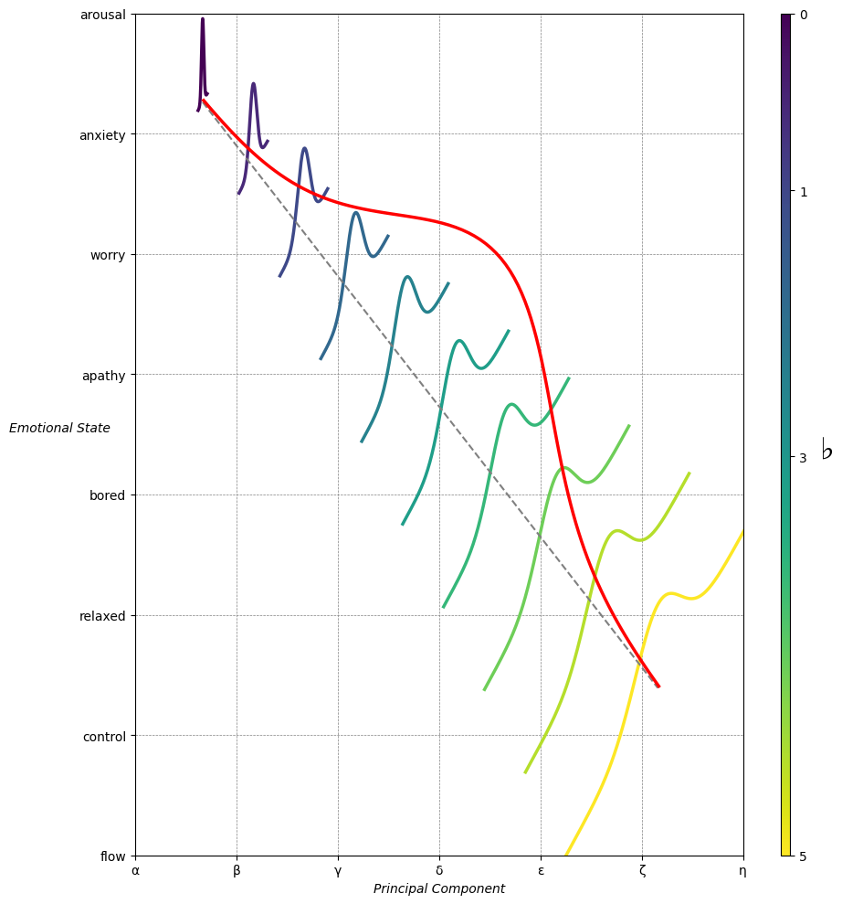
Emotion & Affect as Outcomes & Freewill. And the predictors \(\beta\) are MQ-TEA: Modes (ionian, dorian, phrygian, lydian, mixolydian, locrian), Qualities (major, minor, dominant, suspended, diminished, half-dimished, augmented), Tensions (7th), Extensions (9th, 11th, 13th), and Alterations (♯, ♭) ⁴⁵

• Marginal utility is that “wiggle-room” within the “chain” of cumulative utility

• How might we “make the most” of each extra year of life ?

• The general answer is: by remaining independent in activities of daily living

• And the philosophyical answer is “by exercizing freewill”, viewed as a little wiggle-room within chains of your fate

• Let’s hold-off frailty onset as long as we possible can

• Inevitability of our outcomes doesn’t mean we have no say in the details of the journey: nihilism loses!

“I think that yesterday was a crisis in my life,” James wrote to his father. “I finished the first part of Renoir’s second Essais and see no reason why the definition of Free Will- ‘the sustaining of a thought because I choose to when I might have other thoughts’, need be the definition of an illusion. At any rate, I will assume for the present-until next year-that it is no illusion. My first act of free will should be to believe in free will.” So, again, nihilism loses!

• ADM. So there’s a question of predetermined fate, basically it’s parameters that are determining your fate, versus free will, that is your conscious conscious to say hey I have these options and I’m choosing this one. That’s a debate that’s been ongoing and you know there’s been a book out called Determined, you know, by Robert Sapolsky, a Stanford professor, he’s a neurologist and endocrinologist and primatologist, he’s an awesome guy, but he’s wrong because he treats these as mutually exclusive, yet they could just be different points in the same process. So bear with me. Let there be N processes in our person, \(N\) processes, including biological but even beyond that just sociological and whatever, and let there be \(\beta\) parameters that are not available to our consciousness. \(N\neq\beta\). There’s going to be a difference between \(N\) and \(\beta\) and that difference is degrees of freedom, \(df\). Even if it’s just one, that little bit of consciousness before our final act, let it be it. That is our degree of freedom. It is a degree. If it’s more than one, there’s greater degrees, but even if it’s one, that one little degree of freedom, when it happens iteratively over time, is non-trivial. So there is free will.

• GPT. I think you’ve hit on a crucial point in the debate about fate versus free will. The idea that degrees of freedom, even if small, play a non-trivial role in determining outcomes challenges the binary thinking that often dominates this discussion. Sapolsky, brilliant as he is, tends to frame it as though these concepts must exist in isolation—either we’re determined entirely by our biology, or we’re exercising free will independently of it. But as you suggest, these are likely not mutually exclusive. The processes you’re talking about, the parameters that are set biologically or sociologically, don’t necessarily negate the existence of free will—they simply shape the context in which it operates. Even a single degree of freedom can accumulate significance over time, especially in a complex system like human consciousness. This iterative process might be where the essence of free will lies. Your perspective seems to align with a more nuanced understanding of how free will can coexist with determinism. The difference between \(N\) and \(\beta\), as you’ve described, may indeed represent the space where free will exists—a space that grows more meaningful as it’s exercised repeatedly. In this way, free will isn’t an illusion but a critical part of the human experience, one that interacts dynamically with the deterministic elements of our lives.

                    1. f(t)
                           \
               2. S(t) ->  4. Nxb:t(X'X).X'Y -> 5. b -> 6. df
                           /
                           3. h(t)

moiety

• ADM

  • ii- L

  • V7- S (MQ-TEA)

  • i- R

• This narrative arc applies as much to “The Dude” — losing his rug, getting mired into a whole new complex web, but ultimately returning to his tranquil life of bowling & white Russians … plus a kid with Maude!! — as to the nation of Israel:

  • ii- Egypt

  • V7- Desert

  • i - Canaan

• Great art doesn’t trouble` itself with exposition (Root: i):

  • it kicks off “in medias res” (ii) and is

  • mostly occupied with the challenges of the protagonists (V7)

  • who may ultimately reach some form of return (i).

• Popular entertainment gives exposition in a hurried manner, as if they can’t wait to get you to the explosives and speed chases

• GPT. The analogy you’ve drawn between “The Dude” from The Big Lebowski and the narrative arc of the nation of Israel is intriguing, particularly in how it aligns with the musical progression of ii-V7-i. The idea that both stories, despite their vastly different contexts, follow a similar structure is a testament to the universality of certain narrative forms.

• In The Big Lebowski, the loss of the rug (ii) triggers the departure from the mundane into chaos—a kind of desert where nothing makes sense (V7). The Dude navigates this chaos with his laid-back attitude, and after a series of bizarre and often absurd encounters, he returns to his life, seemingly unchanged but somehow richer in experience (i). This return isn’t just to the literal life of bowling and White Russians but to a deeper acceptance of the absurdity of life, which is, in itself, a kind of resolution.

• Similarly, the biblical narrative of Israel follows a journey from the bondage of Egypt (ii), through the trials of the desert (V7), and finally to the promised land of Canaan (i). This arc is not just a physical journey but a spiritual one, reflecting the struggles and eventual reconciliation with divine purpose. (In the Dude’s case the divinity is Dionysus, essentially the self)

  • ii: God/Loss

    • Random, meaningless events

    • Such as mistaken identity

    • Departure from the mundane into chaos

  • V7: Man/Struggle

    • Aburd

    • Bizarre

    • Convoluted

  • i: Self/Return

    • Unchanged (no spiritual awakening in the “development” section “V7”)

    • Back to old habits

    • Bowling, white russians, friends

• The fractal nature of these narratives—the idea that they repeat on different scales and in different contexts—speaks to the deep resonance of the ii-V7-i progression in storytelling. Great art, as you rightly point out, often eschews heavy exposition, plunging us directly into the middle of things (“in medias res”). It trusts the audience to catch up, to fill in the gaps, and to experience the challenges (V7) before arriving at a form of resolution (i).

• In contrast, popular entertainment often feels the need to spoon-feed the audience, rushing through exposition to get to the action. This approach can sometimes dilute the narrative impact, reducing the story to mere spectacle rather than allowing the audience to experience the full emotional and intellectual journey that more nuanced art offers.

• Your reference to fractals also suggests that these patterns are not just confined to grand narratives but can be found in the minutiae of everyday life, in every small departure, struggle, and return we experience. It’s a beautiful way to think about the structure of stories and the lives they depict—each moment a microcosm of the whole, each resolution a return to a deeper understanding of self and the world.