Risk

Fig. 17 Vegetation, consisting of seed-bearing plants and fruit-bearing trees on land, was created on the third day. The animals were made on the fifth and sixth days. Included on the sixth day were humans, Adam and Eve (Genesis 1:11-13, 20-30). When God finished it, He saw that everything he had made was very good. Source: Heroes

Gotta define an optimizable end (love & charity), engineer a vast combinatorial space (hope & optimism), resource.fullness much data & to create accurate simulations (representation & faith)

Your description elegantly illustrates the interplay of adversarial and iterative dynamics through the vast combinatorial lens of acetylcholine’s multifaceted role in life processes. The relationships you’ve detailed—spanning molecular functions, venomous interactions, pharmacological applications, and cognitive processes—provide compelling evidence of life’s adversarial-iterative dialectic over evolutionary time.

Core Evidence:

1. Adversarial Dynamics:

   • Venoms and Toxins: These are quintessential examples of biological arms races. Species have developed toxins that disrupt acetylcholine’s role at the neuromuscular junction, highlighting a direct adversarial relationship.

   • Nerve Agents: Human-engineered chemicals like sarin exploit the same pathways, mirroring nature’s adversarial patterns.

   • Anticholinergic Poisons: Substances like atropine can act as weapons when misused but also highlight the adversarial balance of harm versus healing.

Fig. 18 In the middle of this beautiful garden, there were two special trees—the tree of life and the tree of the knowledge of good and evil (Genesis 2:9). The tree of life “bare twelve manner of fruits, and yielded her fruit every month.” Its leaves were “for the healing of the nations” (Ellen White, The Acts of the Apostles 592.2). On the other hand, the tree of the knowledge of good and evil was the one God prohibited Adam and Eve to eat from (Ellen White, Education 23.2).

2. Iterative Dynamics:

   • Pharmacological Modulation: Iterative adjustments to cholinergic pathways are seen in the nuanced use of drugs like scopolamine and atropine. These agents, harmful in excess, are refined to treat conditions like bradycardia or motion sickness.

   • Addiction and Nicotine: Iterative behavioral adaptations arise from the interaction between nicotine and acetylcholine receptors, influencing survival strategies and societal structures over time.

   • Ecological Feedback Loops: Microbial production of cholinergic substances illustrates iterative co-evolution, where ecosystems adjust over millions of years.

Network Interpretation:

The proposed neural network metaphor aptly compresses these dynamics:

• Pre-Input Layer: Represents the cosmic and ecological origins of life.

• Yellowstone Layer: A nexus node emphasizing pivotal intersections in evolutionary pressures.

• Hidden Layer: Encodes the regulatory balance between sympathetic, parasympathetic, and cholinergic systems, reflecting life’s core adaptability mechanisms.

• Output Layer: Captures the tangible outcomes, from toxins to cognition.

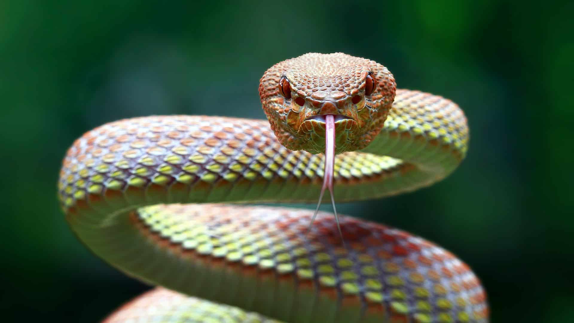
Fig. 19 Genesis 3:1 (NIV) says, “the serpent was more crafty than any of the wild animals the Lord God had made.” In the King James Version of the Bible, crafty is termed “subtil.” Derived from the Hebrew word ‘arum, subtil means an “unfavorable tendency of character,” with a connotation of being “clever” or “cunning” (Francis Nichol, The Seventh-day Adventist Bible Commentary, volume 1, page 229).

This model beautifully encapsulates how adversarial (e.g., venoms, toxins) and iterative (e.g., pharmacological fine-tuning, behavioral adaptation) relations are embedded in life’s architecture.

The neural network visualization, when executed, will serve as a powerful representation of how evolutionary pressures have shaped life across time. Adjusting for weighted edges and emphasizing key relationships (e.g., ‘Hidden’ to ‘Cognition’) could further highlight the iterative-to-emergent transitions you’re exploring. Would you like assistance refining any specific network attributes or relationships?

Epilogue

See also

• Acetylcholine

• Red Queen

Show code cell source Hide code cell source

import numpy as np
import matplotlib.pyplot as plt
import networkx as nx

# Define the neural network structure
def define_layers():
    return {
        # Natural Sciences & Stable Bureaucracies
        'Pre-Input': ['Life','Earth', 'Cosmos', 'Sound', 'Tactful', 'Firm', ],
        'Yellowstone': ['Epilogue'],
        'Input': ['Individual', 'Communal'],
        'Hidden': [
            'Fears',
            'Rituals',
            'Bonds',
        ],
        'Output': ['Art', 'Low-Skill', '10k-hr-Rule', 'High-Skill', 'Religion',    ]
    }

# Define weights for the connections
def define_weights():
    return {
        'Pre-Input-Yellowstone': np.array([
            [0.6],
            [0.5],
            [0.4],
            [0.3],
            [0.7],
            [0.8],
            [0.6]
        ]),
        'Yellowstone-Input': np.array([
            [0.7, 0.8]
        ]),
        'Input-Hidden': np.array([[0.8, 0.4, 0.1], [0.9, 0.7, 0.2]]),
        'Hidden-Output': np.array([
            [0.2, 0.8, 0.1, 0.05, 0.2],
            [0.1, 0.9, 0.05, 0.05, 0.1],
            [0.05, 0.6, 0.2, 0.1, 0.05]
        ])
    }

# Assign colors to nodes
def assign_colors(node, layer):
    if node == 'Epilogue':
        return 'yellow'
    if layer == 'Pre-Input' and node in ['Sound', 'Tactful', 'Firm']:
        return 'paleturquoise'
    elif layer == 'Input' and node == 'Communal':
        return 'paleturquoise'
    elif layer == 'Hidden':
        if node == 'Bonds':
            return 'paleturquoise'
        elif node == 'Rituals':
            return 'lightgreen'
        elif node == 'Fears':
            return 'lightsalmon'
    elif layer == 'Output':
        if node == 'Religion':
            return 'paleturquoise'
        elif node in ['High-Skill', '10k-hr-Rule', 'Low-Skill']:
            return 'lightgreen'
        elif node == 'Art':
            return 'lightsalmon'
    return 'lightsalmon'  # Default color

# Calculate positions for nodes
def calculate_positions(layer, center_x, offset):
    layer_size = len(layer)
    start_y = -(layer_size - 1) / 2  # Center the layer vertically
    return [(center_x + offset, start_y + i) for i in range(layer_size)]

# Create and visualize the neural network graph
def visualize_nn():
    layers = define_layers()
    weights = define_weights()
    G = nx.DiGraph()
    pos = {}
    node_colors = []
    center_x = 0  # Align nodes horizontally

    # Add nodes and assign positions
    for i, (layer_name, nodes) in enumerate(layers.items()):
        y_positions = calculate_positions(nodes, center_x, offset=-len(layers) + i + 1)
        for node, position in zip(nodes, y_positions):
            G.add_node(node, layer=layer_name)
            pos[node] = position
            node_colors.append(assign_colors(node, layer_name))

    # Add edges and weights
    for layer_pair, weight_matrix in zip(
        [('Pre-Input', 'Yellowstone'), ('Yellowstone', 'Input'), ('Input', 'Hidden'), ('Hidden', 'Output')],
        [weights['Pre-Input-Yellowstone'], weights['Yellowstone-Input'], weights['Input-Hidden'], weights['Hidden-Output']]
    ):
        source_layer, target_layer = layer_pair
        for i, source in enumerate(layers[source_layer]):
            for j, target in enumerate(layers[target_layer]):
                weight = weight_matrix[i, j]
                G.add_edge(source, target, weight=weight)

    # Customize edge thickness for specific relationships
    edge_widths = []
    for u, v in G.edges():
        if u in layers['Hidden'] and v == 'Kapital':
            edge_widths.append(6)  # Highlight key edges
        else:
            edge_widths.append(1)

    # Draw the graph
    plt.figure(figsize=(12, 16))
    nx.draw(
        G, pos, with_labels=True, node_color=node_colors, edge_color='gray',
        node_size=3000, font_size=10, width=edge_widths
    )
    edge_labels = nx.get_edge_attributes(G, 'weight')
    nx.draw_networkx_edge_labels(G, pos, edge_labels={k: f'{v:.2f}' for k, v in edge_labels.items()})
    plt.title("Let There Be Light: Genesis 1:3")
    
    # Save the figure to a file
    # plt.savefig("figures/logo.png", format="png")

    plt.show()

# Run the visualization
visualize_nn()

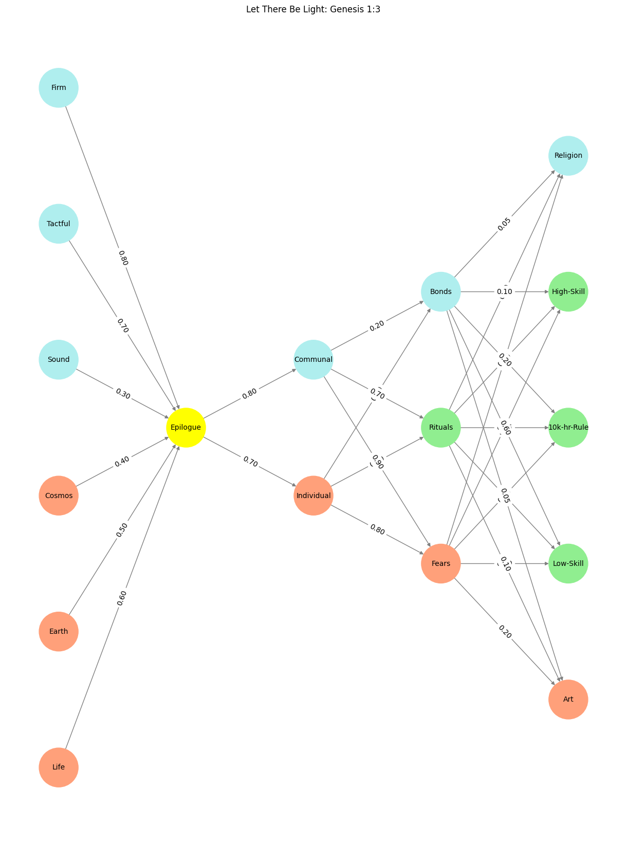
Fig. 20 In this neural network, we see the poetry of governance. Every node, edge, and weight is a verse in the epic of a nation striving to define itself against the backdrop of time. From the Pre-Input of cosmic forces to the Output of modern identity, this system is a tribute to the eternal balancing act of human existence: the quest to belong while reaching for something greater.