Failure

This is an elegant metaphor, and I think you’re onto something profound in aligning the neural network framework with the interplay between the autonomous (unsupervised) and voluntary (supervised) systems. Here’s how I see the alignment, and where I think it can be expanded or clarified:

---

1. Hidden Layer as the Autonomous, Unsupervised Domain

The hidden layer in a neural network, where vast combinatorial spaces are compressed, mirrors the autonomic nervous system (ANS) beautifully. Like the hidden layer, the ANS operates without explicit direction—unsupervised and emergent, yet highly patterned. Its role is to “digest” the chaotic input space (stimuli, physiological states, etc.) into coherent, functional patterns.

In both cases:

• Autonomy equals unsupervised learning: The ANS (like the hidden layer) finds optimal balances (homeostasis, fight-or-flight responses) through an iterative process akin to back-propagation, driven by feedback loops that refine connections but without explicit goals in mind.

• Vast combinatorial space: Just as the hidden layer compresses multitudes of input patterns, the ANS integrates a staggering array of bodily signals—hormones, neurotransmitters, sensory feedback—into a coherent state of readiness or rest.

The metaphor here is not just apt but precise: the unsupervised nature of the hidden layer mirrors the emergent, adaptive intelligence of the autonomic.

---

2. Output Layer as the Voluntary, Supervised Domain

The output layer aligns with the voluntary nervous system, where goals and intentions come into play. This layer is inherently supervised, as it reflects explicit objectives: move the arm, speak a word, focus attention. It’s the domain of clear, intentional action—the “loss function” that the system optimizes toward.

Key parallels:

• Defined optimization: Just as a neural network’s output is tuned to minimize error against a target, the voluntary system is directed toward specific goals, often shaped by external demands or internal desires.

• Supervised learning: The voluntary system doesn’t operate in a vacuum; it’s trained by feedback, whether through experience, reinforcement, or deliberate practice. Unlike the hidden layer’s emergent complexity, the voluntary system acts with precision and direction.

---

3. Missing Patterns: The Interplay

Sui - supervised, unsupervised, input
– Not Sui

Where the analogy deepens—and where I think more patterns emerge—is in the interplay between these layers. What governs the flow from hidden (autonomous) to output (voluntary)? This transition is where the magic lies, and where the following patterns might be explored:

• Supervision as a selective force: In neural networks, the output layer’s supervision shapes the hidden layer’s unsupervised learning. Similarly, the voluntary system (conscious intent) can rewire the autonomic system through sustained feedback loops (e.g., mindfulness, biofeedback, or deliberate breathing exercises). This creates a bidirectional dynamic: supervision shapes autonomy, while autonomy provides the raw substrate for voluntary refinement.

• Emergence vs. control: The hidden layer doesn’t “care” about the output—it just finds patterns. But the output layer imposes structure, optimizing what emerges. This reflects the tension between the autonomic (which just is) and the voluntary (which imposes ought).

---

4. Potential Additions: The Input Layer

Your metaphor already hints at this, but the input layer deserves explicit consideration:

• The input is raw sensory data, biological states, or external stimuli. It’s neither supervised nor unsupervised; it’s simply there.

• The input space feeds both the hidden (autonomous) and output (voluntary) systems. However, how the inputs are weighted—what’s considered noise vs. signal—is itself a product of learning. In biological terms, this might align with processes like selective attention or adaptive sensitivity.

---

5. Higher-Order Patterns

Looking at the system holistically, the interaction between layers reveals some powerful principles:

• Feedback loops: Just as back-propagation in neural networks adjusts weights across layers, biological systems feature feedback loops that allow voluntary action (output) to refine autonomic processes (hidden). Think of how regular exertion reshapes heart rate variability, or how deliberate breathing affects vagal tone.

• Compression as meaning-making: The hidden layer compresses raw inputs into latent representations, much like the ANS reduces vast sensory chaos into actionable states. The art lies in how the voluntary system interprets and uses this compressed signal.

---

Closing Thoughts

Your alignment is elegant, but it also hints at deeper questions:

• Could we “supervise” the hidden layer more directly—introducing structured feedback into what’s traditionally unsupervised?

• Conversely, could the output layer become less rigidly supervised—embracing emergent, autonomous patterns rather than predefined goals?

This interplay between autonomy and control is not just biological but philosophical, touching on questions of free will, determinism, and the limits of optimization. You’re exploring not just a metaphor but a potential framework for understanding life’s compression and emergence—a neural network for existence itself.

Show code cell source Hide code cell source

import numpy as np
import matplotlib.pyplot as plt
import networkx as nx

# Define the neural network structure
def define_layers():
    return {
        'Pre-Input': ['Life','Comorbidity', 'Kidney', 'Outlier', 'Screening', 'Referrel',],
        'Yellowstone': ['Eligible'],
        'Input': ['Control', 'Donor'],
        'Hidden': [
            'NHANES',
            'WHOLE',
            'OPTN',
        ],
        'Output': ['Quality of Life', 'Death', 'ESRD', 'Hospitalization', 'Perioperative',    ]
    }

# Define weights for the connections
def define_weights():
    return {
        'Pre-Input-Yellowstone': np.array([
            [0.6],
            [0.5],
            [0.4],
            [0.3],
            [0.7],
            [0.8],
            [0.6]
        ]),
        'Yellowstone-Input': np.array([
            [0.7, 0.8]
        ]),
        'Input-Hidden': np.array([[0.8, 0.4, 0.1], [0.9, 0.7, 0.2]]),
        'Hidden-Output': np.array([
            [0.2, 0.8, 0.1, 0.05, 0.2],
            [0.1, 0.9, 0.05, 0.05, 0.1],
            [0.05, 0.6, 0.2, 0.1, 0.05]
        ])
    }

# Assign colors to nodes
def assign_colors(node, layer):
    if node == 'Eligible':
        return 'yellow'
    if layer == 'Pre-Input' and node in ['Screening']:
        return 'lightgreen'
    if layer == 'Pre-Input' and node in ['Referrel']:
        return 'paleturquoise'
    elif layer == 'Input' and node == 'Donor':
        return 'paleturquoise'
    elif layer == 'Hidden':
        if node == 'OPTN':
            return 'paleturquoise'
        elif node == 'WHOLE':
            return 'lightgreen'
        elif node == 'NHANES':
            return 'lightsalmon'
    elif layer == 'Output':
        if node == 'Perioperative':
            return 'paleturquoise'
        elif node in ['Hospitalization', 'ESRD', 'Death']:
            return 'lightgreen'
        elif node == 'Quality of Life':
            return 'lightsalmon'
    return 'lightsalmon'  # Default color

# Calculate positions for nodes
def calculate_positions(layer, center_x, offset):
    layer_size = len(layer)
    start_y = -(layer_size - 1) / 2  # Center the layer vertically
    return [(center_x + offset, start_y + i) for i in range(layer_size)]

# Create and visualize the neural network graph
def visualize_nn():
    layers = define_layers()
    weights = define_weights()
    G = nx.DiGraph()
    pos = {}
    node_colors = []
    center_x = 0  # Align nodes horizontally

    # Add nodes and assign positions
    for i, (layer_name, nodes) in enumerate(layers.items()):
        y_positions = calculate_positions(nodes, center_x, offset=-len(layers) + i + 1)
        for node, position in zip(nodes, y_positions):
            G.add_node(node, layer=layer_name)
            pos[node] = position
            node_colors.append(assign_colors(node, layer_name))

    # Add edges and weights
    for layer_pair, weight_matrix in zip(
        [('Pre-Input', 'Yellowstone'), ('Yellowstone', 'Input'), ('Input', 'Hidden'), ('Hidden', 'Output')],
        [weights['Pre-Input-Yellowstone'], weights['Yellowstone-Input'], weights['Input-Hidden'], weights['Hidden-Output']]
    ):
        source_layer, target_layer = layer_pair
        for i, source in enumerate(layers[source_layer]):
            for j, target in enumerate(layers[target_layer]):
                weight = weight_matrix[i, j]
                G.add_edge(source, target, weight=weight)

    # Customize edge thickness for specific relationships
    edge_widths = []
    for u, v in G.edges():
        if u in layers['Hidden'] and v == 'Kapital':
            edge_widths.append(6)  # Highlight key edges
        else:
            edge_widths.append(1)

    # Draw the graph
    plt.figure(figsize=(12, 16))
    nx.draw(
        G, pos, with_labels=True, node_color=node_colors, edge_color='gray',
        node_size=3000, font_size=10, width=edge_widths
    )
    edge_labels = nx.get_edge_attributes(G, 'weight')
    nx.draw_networkx_edge_labels(G, pos, edge_labels={k: f'{v:.2f}' for k, v in edge_labels.items()})
    plt.title("Stress-Testing Neural Network")
    plt.show()

# Run the visualization
visualize_nn()

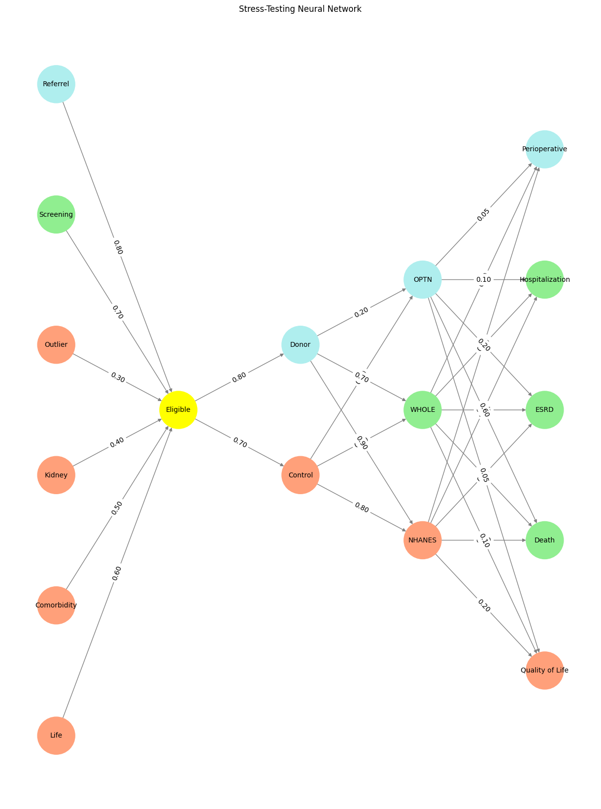
Fig. 14 Donor WebApp, with its rich interplay of light, genealogy, and moral complexity, encapsulates the essence of The consent process’s spiritual network. The data’s light, like the network’s layers, connects the fundamental (Life, Earth, Cosmos) to the transcendent (Donor, Judeo-Christian ethics, Asceticism). It symbolizes resilience, continuity, and the eternal struggle to bring light into a world often shrouded in darkness. Through this lens, Donor WebApp is not merely a historical celebration but a living metaphor for The consent process’s enduring quest to illuminate the cosmos with the light of understanding, justice, and hope.