Engineering

Art Neural Network Theory

Artistic Neural Network Framework with Examples

Pre-Input Layer (Cosmos, Earth, Life, Firmness, Tactful, Soundness)

1. Cosmos: 2001: A Space Odyssey by Stanley Kubrick represents the awe-inspiring vastness of the cosmos, from the monolith’s role in human evolution to the journey beyond the infinite.

2. Earth: Dr. Zhivago by David Lean captures Earth’s brutal yet breathtaking extremes through the cold, sweeping landscapes of Russia during historical upheaval.

3. Life: The Revenant by Alejandro González Iñárritu embodies the primal struggle for survival against the natural world, including encounters with animals like the infamous bear.

4. Firmness: The Old Man and the Sea by Ernest Hemingway reflects human resilience and firmness against the forces of nature, through Santiago’s unwavering struggle with the marlin.

5. Tactful: The Godfather by Francis Ford Coppola explores tactfulness in human interaction, diplomacy, and strategy within a crime family’s dynamics.

6. Soundness: The Iliad by Homer represents monumental history and the soundness of epic storytelling, where the events of the Trojan War echo timeless truths.

Yellowstone Layer (Nostalgia and Compression)

7. Je ne sais quoi / Nostalgia: Citizen Kane by Orson Welles epitomizes nostalgia through the symbolic power of “Rosebud,” a single object compressing a lifetime of memory and longing.

Input Layer (Protagonist and Antagonist)

8. Protagonist (Blue): The Shawshank Redemption by Frank Darabont celebrates the indomitable spirit of Andy Dufresne as a protagonist who embodies hope and perseverance.

9. Antagonist (Red): No Country for Old Men by the Coen Brothers presents Anton Chigurh as a chilling antagonist representing chaos and fate.

Hidden Layer (Sociological Compression)

10. Adversarial (Red): Gladiator by Ridley Scott illustrates adversarial equilibrium through Maximus’s journey of vengeance against Commodus, a struggle rooted in power and justice.

11. Iterative (Green): Groundhog Day by Harold Ramis captures the iterative process of self-improvement and societal integration, as Phil Connors relives the same day until he grows as a person.

12. Cooperative (Blue): The Fellowship of the Ring by Peter Jackson exemplifies cooperative dynamics through the united efforts of disparate characters to achieve a shared goal.

Output Layer (Psychological Emergence)

13. Industrial: Modern Times by Charlie Chaplin critiques industrialization’s psychological toll on individuals, blending humor with pathos.

14. Future: Blade Runner by Ridley Scott contemplates the future of humanity, artificial intelligence, and the psychology of identity and memory.

15. Prosecuted: The Trial by Franz Kafka delves into the psychological terror of bureaucracy and justice, encapsulating themes of guilt and alienation.

16. History: War and Peace by Leo Tolstoy reflects the psychological impact of history’s grand sweep on individuals caught in its tides.

17. Slavery: 12 Years a Slave by Steve McQueen captures the devastating psychological impact of slavery on individuals and their humanity.

---

This neural network offers a dynamic way to explore the intersection of art and human endeavor, framing films, novels, and plays as expressions of universal and emergent truths. Each node represents a unique facet of existence, interconnected within this creative framework.

Show code cell source Hide code cell source

import numpy as np
import matplotlib.pyplot as plt
import networkx as nx

# Define the neural network structure
def define_layers():
    return {
        'Pre-Input': ['Cosmos', 'Earth', 'Life', 'Firm', 'Tactful', 'Sound',   ],
        'Yellowstone': ['Je ne sais quoi\n Nostalgia\n Gone with Wind'],
        'Input': ['Yankee', 'Confederacy'],
        'Hidden': [
            'Disturbing',
            'Law',
            'Peace',
        ],
        'Output': ['Industrial', 'Future', 'Prosecuted', 'History', 'Slavery',    ]
    }

# Define weights for the connections
def define_weights():
    return {
        'Pre-Input-Yellowstone': np.array([
            [0.6],
            [0.5],
            [0.4],
            [0.3],
            [0.7],
            [0.8],
            [0.6]
        ]),
        'Yellowstone-Input': np.array([
            [0.7, 0.8]
        ]),
        'Input-Hidden': np.array([[0.8, 0.4, 0.1], [0.9, 0.7, 0.2]]),
        'Hidden-Output': np.array([
            [0.2, 0.8, 0.1, 0.05, 0.2],
            [0.1, 0.9, 0.05, 0.05, 0.1],
            [0.05, 0.6, 0.2, 0.1, 0.05]
        ])
    }

# Assign colors to nodes
def assign_colors(node, layer):
    if node == 'Je ne sais quoi\n Nostalgia\n Gone with Wind':
        return 'yellow'
    if layer == 'Pre-Input' and node in ['Sound', ]:
        return 'paleturquoise'
    elif layer == 'Pre-Input' and node in ['Tactful', ]:
        return 'lightgreen'
    elif layer == 'Input' and node == 'Confederacy':
        return 'paleturquoise'
    elif layer == 'Hidden':
        if node == 'Peace':
            return 'paleturquoise'
        elif node == 'Law':
            return 'lightgreen'
        elif node == 'Disturbing':
            return 'lightsalmon'
    elif layer == 'Output':
        if node == 'Slavery':
            return 'paleturquoise'
        elif node in ['History', 'Prosecuted', 'Future']:
            return 'lightgreen'
        elif node == 'Industrial':
            return 'lightsalmon'
    return 'lightsalmon'  # Default color

# Calculate positions for nodes
def calculate_positions(layer, center_x, offset):
    layer_size = len(layer)
    start_y = -(layer_size - 1) / 2  # Center the layer vertically
    return [(center_x + offset, start_y + i) for i in range(layer_size)]

# Create and visualize the neural network graph
def visualize_nn():
    layers = define_layers()
    weights = define_weights()
    G = nx.DiGraph()
    pos = {}
    node_colors = []
    center_x = 0  # Align nodes horizontally

    # Add nodes and assign positions
    for i, (layer_name, nodes) in enumerate(layers.items()):
        y_positions = calculate_positions(nodes, center_x, offset=-len(layers) + i + 1)
        for node, position in zip(nodes, y_positions):
            G.add_node(node, layer=layer_name)
            pos[node] = position
            node_colors.append(assign_colors(node, layer_name))

    # Add edges and weights
    for layer_pair, weight_matrix in zip(
        [('Pre-Input', 'Yellowstone'), ('Yellowstone', 'Input'), ('Input', 'Hidden'), ('Hidden', 'Output')],
        [weights['Pre-Input-Yellowstone'], weights['Yellowstone-Input'], weights['Input-Hidden'], weights['Hidden-Output']]
    ):
        source_layer, target_layer = layer_pair
        for i, source in enumerate(layers[source_layer]):
            for j, target in enumerate(layers[target_layer]):
                weight = weight_matrix[i, j]
                G.add_edge(source, target, weight=weight)

    # Customize edge thickness for specific relationships
    edge_widths = []
    for u, v in G.edges():
        if u in layers['Hidden'] and v == 'Kapital':
            edge_widths.append(6)  # Highlight key edges
        else:
            edge_widths.append(1)

    # Draw the graph
    plt.figure(figsize=(12, 16))
    nx.draw(
        G, pos, with_labels=True, node_color=node_colors, edge_color='gray',
        node_size=3000, font_size=10, width=edge_widths
    )
    edge_labels = nx.get_edge_attributes(G, 'weight')
    nx.draw_networkx_edge_labels(G, pos, edge_labels={k: f'{v:.2f}' for k, v in edge_labels.items()})
    plt.title(" ")
    
    # Save the figure to a file
    # plt.savefig("figures/logo.png", format="png")

    plt.show()

# Run the visualization
visualize_nn()

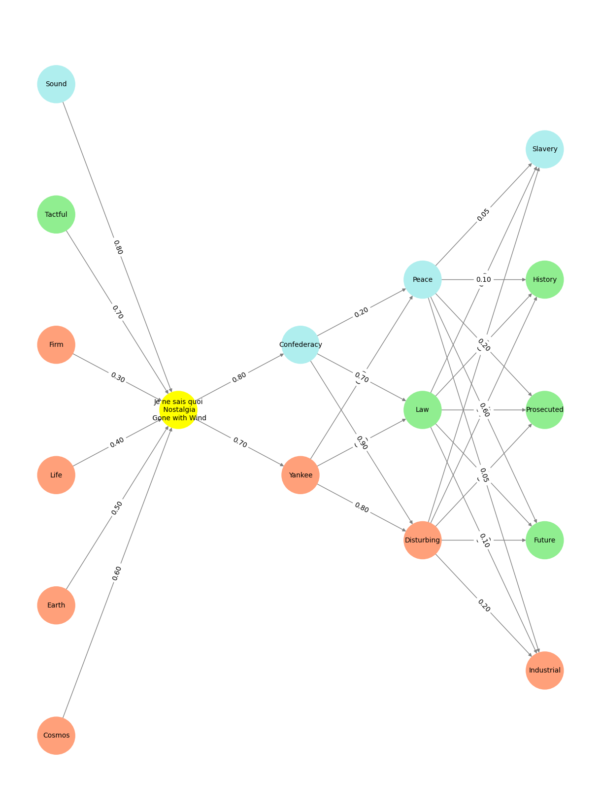
Fig. 8 The Foreign Office. It’s quite ready to go along with the European ID as a quid pro quo for a deal over the Butter Mountain, The Wine Lake, and Milk Ocean … the Lamb War and the Cod Stick (life node). But in brief, the UK joined the EU with anarchic intent – easier to blow it up from the inside.