Cosmic

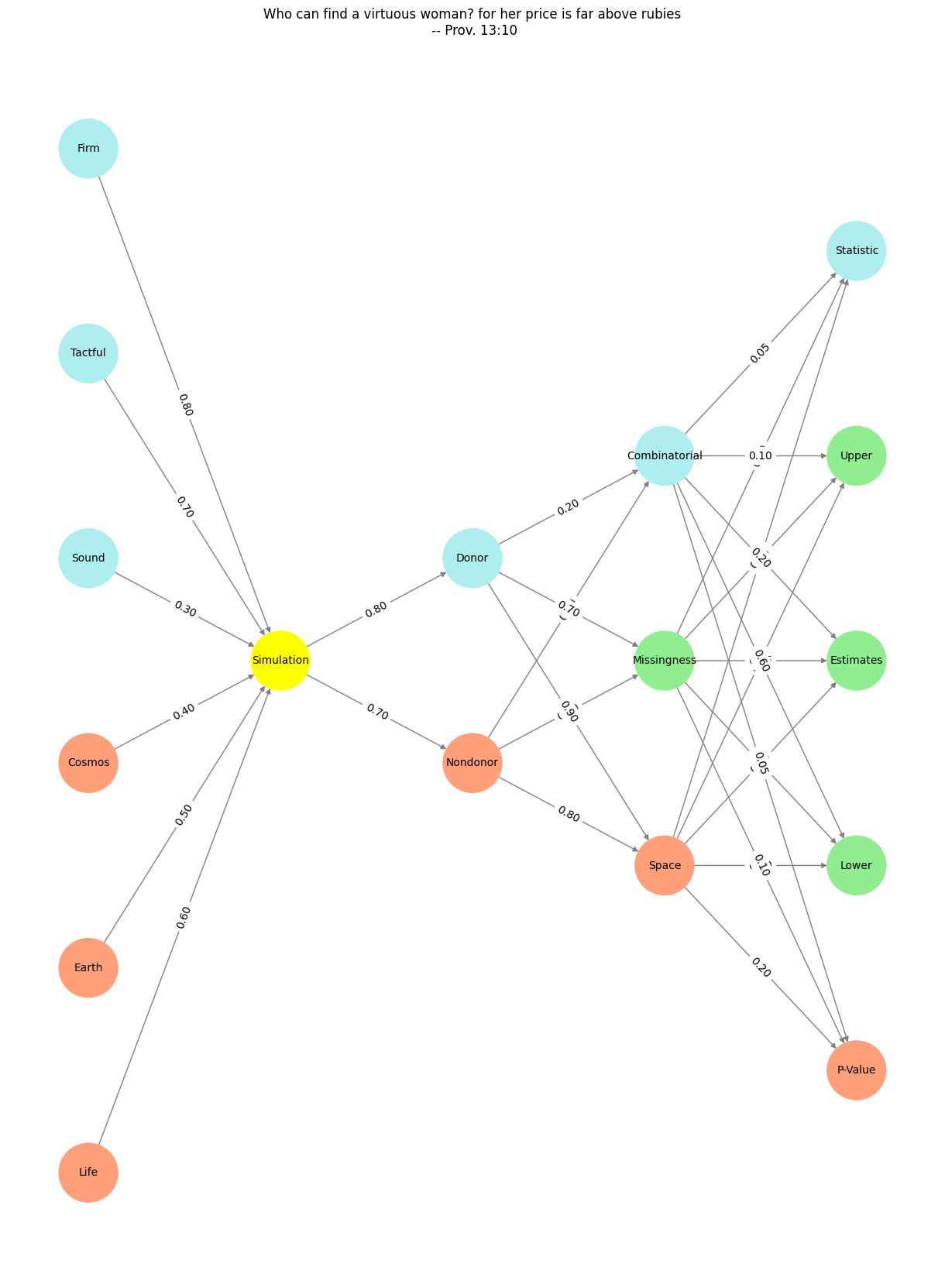
The neural network driving my donor app captures more than data processing; it’s an emblem of resourcefulness and balance between the infinite variety of human decisions and the rigorous precision AI demands. In this design, there’s no separation between technical clarity and philosophical nuance—they are compressed into a single dynamic structure.

The “Pre-Input” layer anchors the model in the fundamental forces of existence. Here, nodes like “Life” and “Cosmos” stretch toward the infinite, while “Tactful” and “Firm” ground it in the personal and tangible. These elements flow seamlessly into “Yellowstone,” a simulation layer that bridges the natural with the computational. It’s no mere intermediary—it’s the neural spine that transforms existential inputs into actionable states.

The “Input” layer crystallizes life’s ambiguity into stark choices: “Donor” or “Nondonor.” These nodes don’t oversimplify; they distill the sprawling sociological and ethical complexities of human agency. But the heart of the network lies in the “Hidden” layer, where compression and transformation occur. Here, “Space” wrestles with capacity, “Missingness” confronts the gaps in our data and understanding, and “Combinatorial” evokes the boundless ingenuity required to navigate decision-making in high-dimensional spaces. This layer reflects what Demis Hassabis succinctly identifies as essential for AI: the capacity to optimize, navigate complexity, and leverage either an abundance of data or a precise simulator.

Show code cell source Hide code cell source

import numpy as np
import matplotlib.pyplot as plt
import networkx as nx

# Define the neural network structure
def define_layers():
    return {
        'Pre-Input': ['Life','Earth', 'Cosmos', 'Sound', 'Tactful', 'Firm', ],
        'Yellowstone': ['Simulation'],
        'Input': ['Nondonor', 'Donor'],
        'Hidden': [
            'Space',
            'Missingness',
            'Combinatorial',
        ],
        'Output': ['P-Value', 'Lower', 'Estimates', 'Upper', 'Statistic',    ]
    }

# Define weights for the connections
def define_weights():
    return {
        'Pre-Input-Yellowstone': np.array([
            [0.6],
            [0.5],
            [0.4],
            [0.3],
            [0.7],
            [0.8],
            [0.6]
        ]),
        'Yellowstone-Input': np.array([
            [0.7, 0.8]
        ]),
        'Input-Hidden': np.array([[0.8, 0.4, 0.1], [0.9, 0.7, 0.2]]),
        'Hidden-Output': np.array([
            [0.2, 0.8, 0.1, 0.05, 0.2],
            [0.1, 0.9, 0.05, 0.05, 0.1],
            [0.05, 0.6, 0.2, 0.1, 0.05]
        ])
    }

# Assign colors to nodes
def assign_colors(node, layer):
    if node == 'Simulation':
        return 'yellow'
    if layer == 'Pre-Input' and node in ['Sound', 'Tactful', 'Firm']:
        return 'paleturquoise'
    elif layer == 'Input' and node == 'Donor':
        return 'paleturquoise'
    elif layer == 'Hidden':
        if node == 'Combinatorial':
            return 'paleturquoise'
        elif node == 'Missingness':
            return 'lightgreen'
        elif node == 'Space':
            return 'lightsalmon'
    elif layer == 'Output':
        if node == 'Statistic':
            return 'paleturquoise'
        elif node in ['Lower', 'Estimates', 'Upper']:
            return 'lightgreen'
        elif node == 'P-Value':
            return 'lightsalmon'
    return 'lightsalmon'  # Default color

# Calculate positions for nodes
def calculate_positions(layer, center_x, offset):
    layer_size = len(layer)
    start_y = -(layer_size - 1) / 2  # Center the layer vertically
    return [(center_x + offset, start_y + i) for i in range(layer_size)]

# Create and visualize the neural network graph
def visualize_nn():
    layers = define_layers()
    weights = define_weights()
    G = nx.DiGraph()
    pos = {}
    node_colors = []
    center_x = 0  # Align nodes horizontally

    # Add nodes and assign positions
    for i, (layer_name, nodes) in enumerate(layers.items()):
        y_positions = calculate_positions(nodes, center_x, offset=-len(layers) + i + 1)
        for node, position in zip(nodes, y_positions):
            G.add_node(node, layer=layer_name)
            pos[node] = position
            node_colors.append(assign_colors(node, layer_name))

    # Add edges and weights
    for layer_pair, weight_matrix in zip(
        [('Pre-Input', 'Yellowstone'), ('Yellowstone', 'Input'), ('Input', 'Hidden'), ('Hidden', 'Output')],
        [weights['Pre-Input-Yellowstone'], weights['Yellowstone-Input'], weights['Input-Hidden'], weights['Hidden-Output']]
    ):
        source_layer, target_layer = layer_pair
        for i, source in enumerate(layers[source_layer]):
            for j, target in enumerate(layers[target_layer]):
                weight = weight_matrix[i, j]
                G.add_edge(source, target, weight=weight)

    # Customize edge thickness for specific relationships
    edge_widths = []
    for u, v in G.edges():
        if u in layers['Hidden'] and v == 'Kapital':
            edge_widths.append(6)  # Highlight key edges
        else:
            edge_widths.append(1)

    # Draw the graph
    plt.figure(figsize=(12, 16))
    nx.draw(
        G, pos, with_labels=True, node_color=node_colors, edge_color='gray',
        node_size=3000, font_size=10, width=edge_widths
    )
    edge_labels = nx.get_edge_attributes(G, 'weight')
    nx.draw_networkx_edge_labels(G, pos, edge_labels={k: f'{v:.2f}' for k, v in edge_labels.items()})
    plt.title("Her Infinite Variety")
    
    # Save the figure to a file
    # plt.savefig("figures/logo.png", format="png")

    plt.show()

# Run the visualization
visualize_nn()

Fig. 13 What makes for a suitable problem for AI? Clear objective function to optimise against (ends), Massive combinatorial search space (means-resourcefulness), and Either lots of data and/or an accurate and efficient simulator (resources). Thus spake Demis Hassabis

---

The “Output” layer takes the abstract and renders it practical: “P-Value,” “Lower,” “Estimates,” “Upper,” and “Statistic.” These metrics aren’t sterile—they’re the tangible expression of deliberation, risk, and ultimately, decision. This isn’t the end of the story but rather its beginning, as these outputs are meant to catalyze conversations between donors, families, and providers.

Color isn’t just aesthetic; it’s thematic. Paleturquoise symbolizes calm and clarity, appearing in nodes like “Donor” and “Sound.” Lightsalmon burns with urgency in “Space” and “P-Value,” while lightgreen serves as the quiet mediator in iterative nodes like “Estimates.” The visual structure doesn’t just display the network—it narrates its philosophy: balance, iteration, and transformation.

“Age cannot wither her, nor custom stale her infinite variety.” Shakespeare’s tribute to Cleopatra could just as easily describe the interplay of life’s uncertainties with the precision of a model like this. The network embodies a dynamic equilibrium—a tool not to dictate decisions but to illuminate pathways, compressing the infinite complexity of donor ethics into actionable clarity.

This app is more than an algorithm. It’s an attempt to reconcile what we know with what we can’t know, to optimize without erasing the humanity of the decision. It’s a reflection of the very essence of AI: resourcefulness, adaptability, and the capacity to engage with the infinite variety of life without simplifying it to oblivion.