
Cunning Strategy#
Here’s a summary of Acts 1 through 4 based on your earlier narrative:
Act 1: The Foundational Study (2010)#
JAMA. 2010 Mar 10;303(10):959-66.
Title: Perioperative Mortality and Long-Term Survival Following Live Kidney Donation.
Key Figures: Dorry L. Segev, Abimereki D. Muzaale, Brian S. Caffo, Shruti H. Mehta, et al. 4
Summary: This landmark study established baseline risks for perioperative mortality (3.1 deaths per 10,000) and showed no significant difference in long-term survival between donors and healthy matched nondonors. It highlighted important demographic differences in risk (e.g., higher in Black donors and those with hypertension).
Impact: With 850 citations, this paper became foundational for live kidney donor safety research, cementing the reputations of Segev, Caffo, and others.
Your Role: As co-author, this was your introduction to academic impact and interdisciplinary collaboration.
Act 2: Expanding the Scope (2014)#
JAMA. 2014 Feb 12;311(6):579-86.
Title: Risk of End-Stage Renal Disease Following Live Kidney Donation.
Key Figures: Abimereki D. Muzaale (first author), Allan B. Massie, Dorry L. Segev, et al. 5
Summary: This study directly addressed a critical gap by comparing ESRD risk in donors with matched healthy nondonors, rather than the general population. Findings revealed that while the absolute risk increase for donors was small, it was higher than for matched nondonors (e.g., 30.8 vs. 3.9 per 10,000 over 15 years).
Impact: With over 1,000 citations, this is your most-cited work, reflecting its groundbreaking methodology and influence on donor counseling practices.
Your Role: As first author, you brought methodological rigor, incorporating control populations to ensure robust comparisons. This paper solidified your reputation in the field.
Act 3: Recent Trends and Methodological Oversights (2024)#
JAMA. 2024 Sep 24;332(12):1015-1017.
Title: Thirty-Year Trends in Perioperative Mortality Risk for Living Kidney Donors.
Key Figures: Allan B. Massie, Dorry L. Segev, et al. 6
Summary: This study aimed to characterize temporal trends in perioperative mortality for kidney donors, focusing on improvements in surgical techniques and donor selection. However, it lacked a control group, limiting its ability to contextualize the observed risks.
Impact: While methodologically limited, the study highlights advances in donor safety but raises questions about the rigor of its design.
Your Role: Although not directly involved, your prior work underscores the importance of including control populations—an omission that could have been addressed had you been consulted.
Act 4: The App Emerges (2025)#
Nephrectomy-Attributable Risk Refinement (Your Thesis Framework).
Abstract: Building upon the 2024 JAMA study, this act introduces your app as a solution to longstanding methodological challenges. By integrating control populations into risk estimation workflows, your app demonstrates how nephrectomy-attributable risks (e.g., 0.9 per 10,000 for young donors) can be quantified with precision.
Key Insight: For older donors, risks may be even lower, but current data gaps hinder accurate estimation. The app addresses these gaps, offering real-time integration of registry data (NHANES, OPTN/SRTR) and advanced statistical models.
Impact: This act reframes the research landscape, showcasing the app’s potential to standardize and refine risk estimation processes in donor evaluations.
Your Role: As the app’s architect, you introduce a paradigm shift in how donor risks are evaluated and communicated.
Themes and Narrative Progression#
Act 1 establishes the foundation of donor safety research.
Act 2 expands the scope with methodological rigor.
Act 3 highlights both progress and persistent methodological shortcomings.
Act 4 introduces your app as the solution, leveraging machine learning principles to address systemic inefficiencies.
These acts collectively set the stage for Act 5, where you present your app as the bridge to a reflexive, iterative future in academic medicine. Let me know if you’d like any further clarification!
Show code cell source
import numpy as np
import matplotlib.pyplot as plt
import networkx as nx

# Define the neural network structure; modified to align with "Aprés Moi, Le Déluge" (i.e. Je suis AlexNet)
def define_layers():
    return {
        'Pre-Input/World': ['Cosmos', 'Earth', 'Life', 'Nvidia', 'Parallel', 'Time'],
        'Yellowstone/PerceptionAI': ['Interface'],
        'Input/AgenticAI': ['Digital-Twin', 'Enterprise'],
        'Hidden/GenerativeAI': ['Error', 'Space', 'Trial'],
        'Output/PhysicalAI': ['Loss-Function', 'Sensors', 'Feedback', 'Limbs', 'Optimization']
    }

# Assign colors to nodes
def assign_colors(node, layer):
    if node == 'Interface':
        return 'yellow'
    if layer == 'Pre-Input/World' and node in [ 'Time']:
        return 'paleturquoise'
    if layer == 'Pre-Input/World' and node in [ 'Parallel']:
        return 'lightgreen'
    elif layer == 'Input/AgenticAI' and node == 'Enterprise':
        return 'paleturquoise'
    elif layer == 'Hidden/GenerativeAI':
        if node == 'Trial':
            return 'paleturquoise'
        elif node == 'Space':
            return 'lightgreen'
        elif node == 'Error':
            return 'lightsalmon'
    elif layer == 'Output/PhysicalAI':
        if node == 'Optimization':
            return 'paleturquoise'
        elif node in ['Limbs', 'Feedback', 'Sensors']:
            return 'lightgreen'
        elif node == 'Loss-Function':
            return 'lightsalmon'
    return 'lightsalmon'  # Default color

# Calculate positions for nodes
def calculate_positions(layer, center_x, offset):
    layer_size = len(layer)
    start_y = -(layer_size - 1) / 2  # Center the layer vertically
    return [(center_x + offset, start_y + i) for i in range(layer_size)]

# Create and visualize the neural network graph
def visualize_nn():
    layers = define_layers()
    G = nx.DiGraph()
    pos = {}
    node_colors = []
    center_x = 0  # Align nodes horizontally

    # Add nodes and assign positions
    for i, (layer_name, nodes) in enumerate(layers.items()):
        y_positions = calculate_positions(nodes, center_x, offset=-len(layers) + i + 1)
        for node, position in zip(nodes, y_positions):
            G.add_node(node, layer=layer_name)
            pos[node] = position
            node_colors.append(assign_colors(node, layer_name))

    # Add edges (without weights)
    for layer_pair in [
        ('Pre-Input/World', 'Yellowstone/PerceptionAI'), ('Yellowstone/PerceptionAI', 'Input/AgenticAI'), ('Input/AgenticAI', 'Hidden/GenerativeAI'), ('Hidden/GenerativeAI', 'Output/PhysicalAI')
    ]:
        source_layer, target_layer = layer_pair
        for source in layers[source_layer]:
            for target in layers[target_layer]:
                G.add_edge(source, target)

    # Draw the graph
    plt.figure(figsize=(12, 8))
    nx.draw(
        G, pos, with_labels=True, node_color=node_colors, edge_color='gray',
        node_size=3000, font_size=10, connectionstyle="arc3,rad=0.1"
    )
    plt.title("Archimedes", fontsize=15)
    plt.show()

# Run the visualization
visualize_nn()
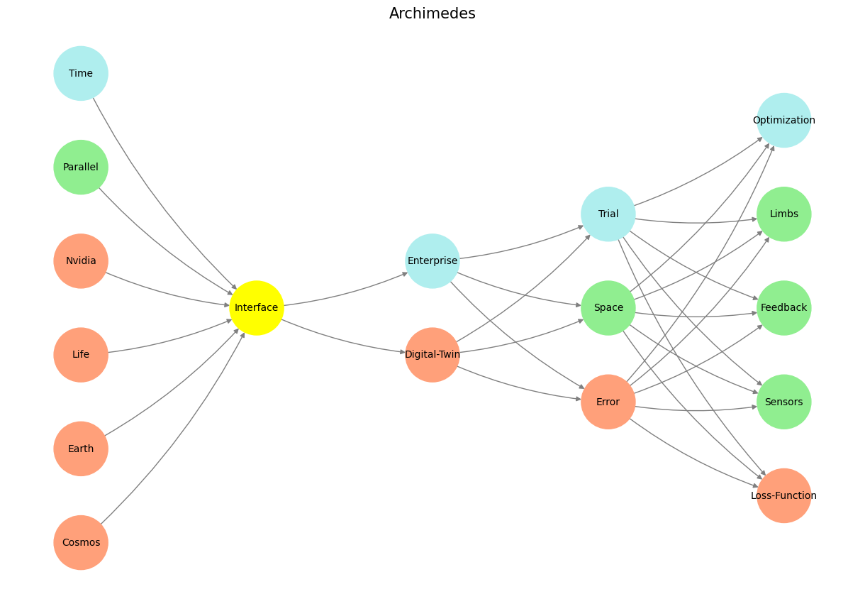

Fig. 7 Nostalgia & Romanticism. When monumental ends (victory), antiquarian means (war), and critical justification (bloodshed) were all compressed into one figure-head: hero#