Duality

Show code cell source Hide code cell source

import matplotlib.pyplot as plt
import networkx as nx

# Function to create the CoffeeTree network with colored edges
def create_colored_coffee_network():
    G = nx.DiGraph()

    # Add edges with color attributes
    edges = [
        ("Coffee", "Drip", "lightblue"),  # Drip branch
        ("Coffee", "Espresso", "lightgreen"),  # Espresso branch
        ("Drip", "Blonde Roast", "lightblue"),
        ("Drip", "Pike Place", "lightblue"),
        ("Drip", "Dark Roast", "lightblue"),
        ("Espresso", "Espresso (Solo/Doppio)", "lightgreen"),
        ("Espresso", "Americano", "lightgreen"),
        ("Espresso", "Custom Made", "lightgreen"),
        ("Custom Made", "Latte", "lightpink"),
        ("Custom Made", "Cappuccino", "lightpink"),
        ("Custom Made", "Macchiato", "lightpink"),
    ]

    for source, target, color in edges:
        G.add_edge(source, target, color=color)

    return G

# Function to extract edge colors for visualization
def get_edge_colors(G):
    return [G[u][v]['color'] for u, v in G.edges]

# Create the network with colored edges
coffee_network = create_colored_coffee_network()

# Plot the network with specified colors
plt.figure(figsize=(12, 8))

# Set a fixed seed for layout consistency
pos = nx.spring_layout(coffee_network, seed=3)  

# Get edge colors for plotting
edge_colors = get_edge_colors(coffee_network)

# Draw the network
nx.draw(
    coffee_network,
    pos,
    with_labels=True,
    node_color="white",
    node_size=3000,
    font_size=10,
    font_weight="bold",
    edge_color=edge_colors,
    arrowsize=20,
    width=2
)

# Add a title to the diagram
plt.title("Starbucks")
plt.show()

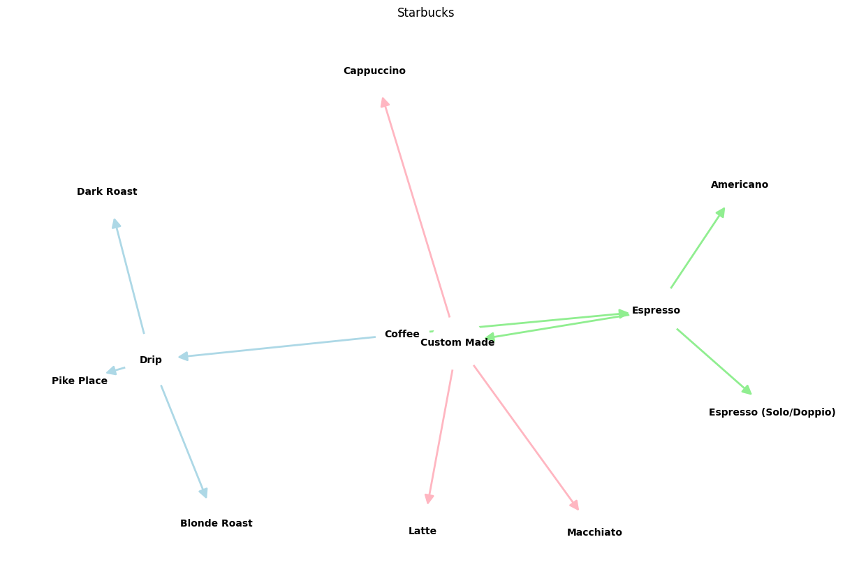
Fig. 13 Leveraged Agency. At Championship-level, tactical approaches aren’t going to win you the trophy. The odds here are 1000/1 or longer and can’t be collapsed, given the numerous entrants and exists each year – similar to what we witnessed in leveraged agency sort of games like horse-racing. The higher the risk, higher the error, because no amount of analysis can ever utilize the most up-to-date dataset when the very populations of study are so dynamic.

Show code cell source Hide code cell source

import numpy as np
import matplotlib.pyplot as plt
import networkx as nx

# Define the neural network fractal
def define_layers():
    return {
        'World': ['Particles-Compression', 'Vibration-Particulate.Matter', 'Ear, Cerebellum-Georientation', 'Harmonic Series-Agency.Phonology', 'Space-Verb.Syntax', 'Time-Object.Meaning', ], # Resources
        'Perception': ['Rhythm, Pockets'], # Needs
        'Agency': ['Open-Nomiddleman', 'Closed-Trusted'], # Costs
        'Generative': ['Ratio-Weaponized', 'Competition-Tokenized', 'Odds-Monopolized'], # Means
        'Physical': ['Volatile-Revolutionary', 'Unveiled-Resentment',  'Freedom-Dance in Chains', 'Exuberant-Jubilee', 'Stable-Conservative'] # Ends
    }

# Assign colors to nodes
def assign_colors():
    color_map = {
        'yellow': ['Rhythm, Pockets'],
        'paleturquoise': ['Time-Object.Meaning', 'Closed-Trusted', 'Odds-Monopolized', 'Stable-Conservative'],
        'lightgreen': ['Space-Verb.Syntax', 'Competition-Tokenized', 'Exuberant-Jubilee', 'Freedom-Dance in Chains', 'Unveiled-Resentment'],
        'lightsalmon': [
            'Ear, Cerebellum-Georientation', 'Harmonic Series-Agency.Phonology', 'Open-Nomiddleman', 
            'Ratio-Weaponized', 'Volatile-Revolutionary'
        ],
    }
    return {node: color for color, nodes in color_map.items() for node in nodes}

# Calculate positions for nodes
def calculate_positions(layer, x_offset):
    y_positions = np.linspace(-len(layer) / 2, len(layer) / 2, len(layer))
    return [(x_offset, y) for y in y_positions]

# Create and visualize the neural network graph
def visualize_nn():
    layers = define_layers()
    colors = assign_colors()
    G = nx.DiGraph()
    pos = {}
    node_colors = []

    # Add nodes and assign positions
    for i, (layer_name, nodes) in enumerate(layers.items()):
        positions = calculate_positions(nodes, x_offset=i * 2)
        for node, position in zip(nodes, positions):
            G.add_node(node, layer=layer_name)
            pos[node] = position
            node_colors.append(colors.get(node, 'lightgray'))  # Default color fallback

    # Add edges (automated for consecutive layers)
    layer_names = list(layers.keys())
    for i in range(len(layer_names) - 1):
        source_layer, target_layer = layer_names[i], layer_names[i + 1]
        for source in layers[source_layer]:
            for target in layers[target_layer]:
                G.add_edge(source, target)

    # Draw the graph
    plt.figure(figsize=(12, 8))
    nx.draw(
        G, pos, with_labels=True, node_color=node_colors, edge_color='gray',
        node_size=3000, font_size=8, connectionstyle="arc3,rad=0.2"
    )
    plt.title("Music", fontsize=13)
    plt.show()

# Run the visualization
visualize_nn()

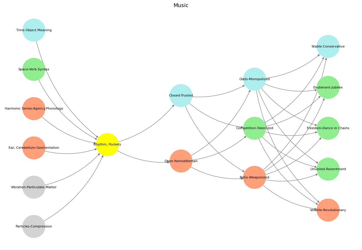
Fig. 14 Tryptophan, Tryptamine, and Y’all Who Be Trippin’. Information in nature is encoded in gravity and photons and zapped from the cosmos, to earth, to life, to silicon. As for the point of view, thats open for discourse. Source: Lorenzo Expeditions. And if we invert all the aforementioned, then we might say something like: The code provides a unique blend of art and science, creating a visual narrative that might engage viewers in thinking about the structure of thought, decision-making, or the whimsical nature of reality as depicted in “Alice’s Adventures in Wonderland” - Grok-2.