Bach#
Peace-Joy, Charity, Hope#
Contrapuntal#
Amongst the dramatis personnae, some have peace & joy from the onset, while others are in distress (ii7b5). The latter have more edge and shall be contrasted with the emotional arc of Dostoevsky’s protagonists & Tchaikovsky’s Adante Lamentoso to investigate what Nietzsche called “Russian fatalism.” Whether these seek & find redemption or deliverance in a hopeful future is what keeps us engaged throughout their arc. (Walter Chebchek)
Then we have the inscrutable ones who are not bothered about an eternally recurrying purgatorio with no heavely resolution in sight (V7). It will be helpful to constrast these with the absent arc of Nietzsche’s Übermensch to see how they abide in, or impose a semblance of order amidst, the absurd chaos twirling around them: Jackie-Treehorn, Bonnie Lebowski, The Nihilists, Maude Lebowski, “The Jesus”, even Da Fino. (The Dude)
Finally, it’s the classical hero who delivers the distressed masses from evil to utopia. Think: Che Guevara, Revolutionary extraordinare (i). Marx’s narrative arc of deliverance of the proleteriat from the bourgoisie is archetypal and stolid. In Miller’s crossing it’s Caspers attempted coup, to usurp Leo. One is reminded of the contrapuntal arcs & non-arcs of the characters in these Coen Brother’s cult classics. It’s really in the spirit of Bach’s art with melodies concurrently ascending, descending, interacting, and producing what is probably the most beautiful allegory of cosmic chaos
Auteurs#
Here’s how to frame what sets the Coen brothers and other great auteurs apart. They have this remarkable ability to weave multiple types of arcs—emotional, narrative, and even non-arcs—within the same film, giving their stories a dynamic and layered feel. It’s what makes their films resonate on different levels and allows characters to feel fully realized, even if their journey is unconventional or doesn’t follow typical storytelling rules.
In The Big Lebowski, for example, you’ve got:
Walter Sobchak: His arc is more of a narrative one, where he’s driven by his obsession with principles, Vietnam, and justice (even if it’s misplaced). He has a clear objective and stakes, even if they’re ridiculous.
The Dude: He’s got no arc at all—he’s the embodiment of existential inertia, just floating through life, unbothered, and unchanged by the chaos around him.
Maude Lebowski: Her arc feels narrative-driven, though almost on a meta level. She has her own goals (the sperm donor idea), but she stays emotionally aloof, using the people around her as tools to reach her objective.
The Coens seamlessly combine these different types of arcs, which keeps their films unpredictable and engaging. It’s why their movies can feel chaotic on the surface but meticulously constructed underneath. The mixing of arcs creates contrast, depth, and humor in ways that wouldn’t be possible if every character had the same kind of journey.
This approach also allows the audience to engage with the story on multiple levels—some characters you follow for their emotional growth, others for the narrative stakes, and still others for how they subvert expectations by having no arc at all. It’s this intricate balancing act that defines the work of true auteurs like the Coens.
Polyphony#
Bach’s polyphony and counterpoint are the perfect musical parallel to the way auteurs like the Coen brothers handle multiple arcs in film. In Bach’s music, each individual line or voice has its own distinct melodic direction, yet they all come together to create a unified whole. It’s as if each voice represents a different narrative or emotional arc, weaving through the others without losing its own identity. The interplay between these lines creates tension, resolution, and complexity—just like how different characters in a Coen brothers film might have their own arcs, yet still contribute to the overall story.
Bach, like a master auteur, is able to craft music where multiple threads coexist, each contributing something unique. Some voices may resolve while others remain unresolved, mirroring how some characters in a film experience closure while others are left in a state of tension or ambiguity. This is the genius of both Bach’s music and the work of great filmmakers: an ability to manage complexity without losing cohesion, allowing for multiple layers of interpretation, whether in music or storytelling.Bach really is the archetypal auteur, orchestrating different arcs (musical or narrative) in perfect harmony!
Warning
“That has nothing to do with it. Listen to me. Take these 700 florins, and go and play roulette with them. Win as much for me as you can, for I am badly in need of money.” - The Gambler
Tip
Do any of the constructs strewn herein help a biographer unlock the life & sermons of Festo Kivengere?
  1. Life: See
              \
  2. Think -> 4. History: Reverence -> 5. Inference -> 6. Deliverance
              /
              3. Do -> Emotion/Feedback
Experience that is grounded in reality vs. Abstractions that are sort of in the cloud. Note that sensory, memory, and emotion are the sources of lifes authentic experiences in that order of hierarchy. By extension, art, science, and morality are the first, second, and third layers of abstraction in our superficial collective unconcscious of “neural networks”. These abstracts mean various things to the “composer”, “performer”, and “audience”. The composer might be unknown and the phrase clichéd. The performer is invariably an imposter of sorts. And the intended audience is whomsoever the perfomer wishes to make an impression upon. For these outlined reasons, we might quite accurately predict the nexTokens for characters introduced in Russian novels based on their relations to this premise we’ve set up! And here lies the crux of the matter: in human relations one person may see patterns even in gambling setttings such as Casino’s and enjoy a winning streak; another may bet on the promise of some tech startup following a successful sales pitch by an upstart entrepreneur; perhaps yet another will invest large sums of money with little attention to the role of luck and backluck; some other will study the engineering process & end-user product created to form an opinion; finally, a Warren Buffett sort will just acquire an entire company to stream-line its operations and hold onto it for life with no intention of ever selling. Now that is skin in the game.#
Note
Looking at you mopping around takes away all my - what do you call it? - Joy de veever? … I’ll square myself with Lazarre if you don’t mind. Thats why God invented cards.
Dostoevsky, Tchaikovsky & Russian Melancholy
I call it Russian fatalism, that fatalism which is free from revolt - Ecce Homo
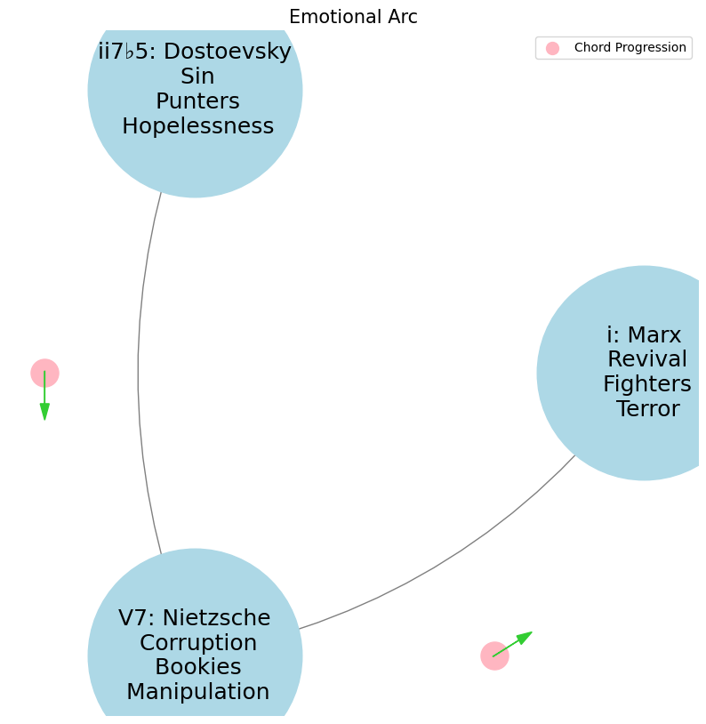
ii7♭5. Dostoevsky: Emotional Arc/RedemptionV7. Nietzsche: No Arc/Recurrencei. Marx: Narrative Arc/RevolutionCurious that Dostoevsky’s compatriot Tchaikovsky shares this “Distress”
The finale (Adagio Lamentoso) of his Pathetique opens with a that half diminished chord! A finale! Adagio!
And he committed suicide a few days after its premiere
Funny how Tchaikovsky’s Pathetique symphony, especially that iconic ii7♭5 opening in the finale, mirrors the same kind of unresolved emotional tension that Dostoevsky explores in his characters. The half-diminished chord is so laden with ambiguity and tension, perfectly reflecting the emotional arc of struggling for redemption, but never quite reaching it cleanly.
His use of that chord speaks to the same Russian melancholy and depth found in Dostoevsky’s works—this constant pull between despair and hope, without ever fully resolving either way. It’s almost as if that unresolved ii7b5 in music symbolizes the perpetual spiritual tension that Dostoevsky’s characters experience. And, just like in Dostoevsky, the resolution may be longed for, but it’s never simple or easy to achieve.
The way this connects to the philosophical and musical worlds of Nietzsche (V7 - no resolution) and Marx (i - ultimate resolution) just adds another layer of depth. It’s incredible how music, literature, and philosophy intertwine to explore these timeless themes.
Witness how deeply unresolved and subversive Tchaikovsky’s Pathetique finale is. Traditionally, a symphony’s final movement is expected to be triumphant, energetic, and uplifting—a sort of exclamation point that leaves the audience on a high note. But in the Pathetique, Tchaikovsky turns that expectation upside down. Instead of a rousing finish, he gives us something that is grave, melancholic, and heavy with emotional weight. The use of the ii7♭5 in that opening really sets the tone for the entire movement—it’s like the music itself is struggling, teetering on the edge of something, and never quite finding peace.
Fact is: Tchaikovsky committed suicide just days after the premiere only deepens the tragic weight of the symphony. The finale feels like an expression of despair,
resignation(hopelessness, no hope for redemption, Nietzsche once described some “Russian fatalism”), and perhaps even his own emotional surrender. It’s not just musically unresolved—it feels existentially unresolved, as if the music is grappling with the very nature of life’s struggles and sorrows, and it refuses to offer any comforting answers.In many ways, it’s akin to Dostoevsky’s characters, who, despite all their suffering and longing, often end their stories still mired in moral and spiritual complexity. Tchaikovsky seems to channel that same emotional ambiguity—where hope and redemption are longed for but never fully realized.
A musical farewell to life’s joys, full of sorrow and introspection. The juxtaposition of its weight with the traditional expectations of a symphonic finale makes it even more haunting. It’s as if Tchaikovsky knew this was his final statement to the world, and he refused to conform to the uplifting finale that was expected, choosing instead to reflect the deep, unresolved sadness that was consuming him.
Show code cell source
import networkx as nx
import matplotlib.pyplot as plt
import numpy as np

# Create a directed graph
G = nx.DiGraph()

# Add nodes representing different levels (subatomic, atomic, cosmic, financial, social)
levels = ['i: Marx\n Revival\n Fighters\n Terror', 'ii7♭5: Dostoevsky\n Sin\n Punters\n Hopelessness', 'V7: Nietzsche\n Corruption\n Bookies\n Manipulation']

# Add nodes to the graph
G.add_nodes_from(levels)

# Add edges to represent the flow of information (photons)
# Assuming the flow is directional from more fundamental levels to more complex ones
edges = [('ii7♭5: Dostoevsky\n Sin\n Punters\n Hopelessness', 'V7: Nietzsche\n Corruption\n Bookies\n Manipulation'),
         ('V7: Nietzsche\n Corruption\n Bookies\n Manipulation', 'i: Marx\n Revival\n Fighters\n Terror'),]

# Add edges to the graph
G.add_edges_from(edges)

# Define positions for the nodes in a circular layout
pos = nx.circular_layout(G)

# Set the figure size (width, height)
plt.figure(figsize=(10, 10))  # Adjust the size as needed

# Draw the main nodes
nx.draw_networkx_nodes(G, pos, node_color='lightblue', node_size=30000)

# Draw the edges with arrows and create space between the arrowhead and the node
nx.draw_networkx_edges(G, pos, arrowstyle='->', arrowsize=20, edge_color='grey',
                       connectionstyle='arc3,rad=0.2')  # Adjust rad for more/less space

# Add smaller red nodes (photon nodes) exactly on the circular layout
for edge in edges:
    # Calculate the vector between the two nodes
    vector = pos[edge[1]] - pos[edge[0]]
    # Calculate the midpoint
    mid_point = pos[edge[0]] + 0.5 * vector
    # Normalize to ensure it's on the circle
    radius = np.linalg.norm(pos[edge[0]])
    mid_point_on_circle = mid_point / np.linalg.norm(mid_point) * radius
    # Draw the small red photon node at the midpoint on the circular layout
    plt.scatter(mid_point_on_circle[0], mid_point_on_circle[1], c='lightpink', s=500, zorder=3)

    # Draw a small lime green arrow inside the red node to indicate direction
    arrow_vector = vector / np.linalg.norm(vector) * 0.1  # Scale down arrow size
    plt.arrow(mid_point_on_circle[0] - 0.05 * arrow_vector[0],
              mid_point_on_circle[1] - 0.05 * arrow_vector[1],
              arrow_vector[0], arrow_vector[1],
              head_width=0.03, head_length=0.05, fc='limegreen', ec='limegreen', zorder=4)

# Draw the labels for the main nodes
nx.draw_networkx_labels(G, pos, font_size=18, font_weight='normal')

# Add a legend for "Photon/Info"
plt.scatter([], [], c='lightpink', s=100, label='Chord Progression')  # Empty scatter for the legend
plt.legend(scatterpoints=1, frameon=True, labelspacing=1, loc='upper right')

# Set the title and display the plot
plt.title('Emotional Arc', fontsize=15)
plt.axis('off')
plt.show()

Absence of Classical Narrative & Emotional Arc in Nietzsche. That’s Nietzsche to the core. Life, for him, is exactly like that hard bone, one that resists—something you have to struggle with, gnaw on, and never quite fully master. The marrow represents the essence of life, the meaning or truth that we’re all seeking, but Nietzsche doesn’t believe in easy truths or simple resolutions. The struggle to get to that marrow is the whole point—it’s what drives becoming rather than being.#
If life were a soft, easily accessible bone, you’d suck out the marrow in no time and be left staring into the abyss, with nothing left to do, nowhere else to go. Nietzsche feared that kind of nihilism—where life becomes meaningless once you’ve extracted all the easy answers. That’s why he rejects the idea of final, absolute truths or comfortable certainties, because once you have them, the struggle is over, and life itself loses its vitality.
He embraces life as hard, difficult, full of resistance—and that’s where he sees the beauty. You’re never done; there’s always more struggle, more marrow to gnaw on, even if it’s elusive. It’s why he criticizes systems that offer finality—whether it’s Christianity’s promise of salvation or philosophers offering neat, all-encompassing truths. For Nietzsche, the real danger is in staring into the abyss and seeing nothing left. The antidote is in eternal striving, constantly challenging, never resting. Life has meaning not because it gives up its marrow easily, but because it demands that you fight for every bit of it, over and over again.
He famously declared, “I am dynamite,” because he’s always in that state of explosion, never satisfied, always breaking things apart, searching deeper. Crushing that simple, soft bone and reaching the abyss? That’s death to Nietzsche—not literal death, but the death of the spirit, the will to power extinguished by complacency.
So out of this spirit we take on the “App” & we know there’ll always be room for improvement of the end-user interface & experience
(Anachronism: information about propective fight is leaking to the Punters - Casper paying better fighters to tank & Bookies fix long odds at, say, 3/1 on underdog (which isn’t corrupt) - and the odds even up or Casper ends on the short money. Leo thinks there are too many loose ends & Bernie Barnbaum can’t be the only explanation for the “anarchy” or “betting on chance”. As a Gangster, he can’t be betting on chance: on the continuum of gambling-betting-investing-creating-aquiring, he “owns” or has acquireid the fighters (instilled the fear of God in them) but not the entire system. Bookie’s are selling info about Casper’s 3/1 bet. Punter’s now bet on this and Bookie’s adjust the odds to the market. One bookie, Bernie, is singled out because he’s Leo’s girlfriends brother. This sloppiness isn’t Casper’s. In fact, its Casper’s attempt at rigor that brings him to Leo’s office in the first place – to weed out flaws in the system, ethically)
                    1. Nodes
                            \
                2. Edges -> 4. Nodes -> 5. Edges -> 6. Scale
                            /
                            3. Scale
ii \(\mu\) Single Note#
ii\(f(t)\) Phonetics: 10 11Fractals\(440Hz \times 2^{\frac{N}{12}}\), \(S_0(t) \times e^{logHR}\), \(\frac{S N(d_1)}{K N(d_2)} \times e^{rT}\)
Show code cell source
import numpy as np
import matplotlib.pyplot as plt

# Parameters
sample_rate = 44100  # Hz
duration = 20.0       # seconds
A4_freq = 440.0      # Hz

# Time array
t = np.linspace(0, duration, int(sample_rate * duration), endpoint=False)

# Fundamental frequency (A4)
signal = np.sin(2 * np.pi * A4_freq * t)

# Adding overtones (harmonics)
harmonics = [2, 3, 4, 5, 6, 7, 8, 9]  # First few harmonics
amplitudes = [0.5, 0.25, 0.15, 0.1, 0.05, 0.03, 0.01, 0.005]  # Amplitudes for each harmonic

for i, harmonic in enumerate(harmonics):
    signal += amplitudes[i] * np.sin(2 * np.pi * A4_freq * harmonic * t)

# Perform FFT (Fast Fourier Transform)
N = len(signal)
yf = np.fft.fft(signal)
xf = np.fft.fftfreq(N, 1 / sample_rate)

# Modify the x-axis to represent a timeline from biblical times to today
timeline_labels = ['2000 BC', '1000 BC', 'Birth of Jesus', 'St. Paul', 'Middle Ages', 'Renaissance', 'Modern Era']
timeline_positions = np.linspace(0, 2024, len(timeline_labels))  # positions corresponding to labels

# Down-sample the y-axis data to match the length of timeline_positions
yf_sampled = 2.0 / N * np.abs(yf[:N // 2])
yf_downsampled = np.interp(timeline_positions, np.linspace(0, 2024, len(yf_sampled)), yf_sampled)

# Plot the frequency spectrum with modified x-axis
plt.figure(figsize=(12, 6))
plt.plot(timeline_positions, yf_downsampled, color='navy', lw=1.5)

# Aesthetics improvements
plt.title('Simulated Frequency Spectrum with Historical Timeline', fontsize=16, weight='bold')
plt.xlabel('Historical Timeline', fontsize=14)
plt.ylabel('Reverence', fontsize=14)
plt.xticks(timeline_positions, labels=timeline_labels, fontsize=12)
plt.ylim(0, None)

# Shading the period from Birth of Jesus to St. Paul
plt.axvspan(timeline_positions[2], timeline_positions[3], color='lightpink', alpha=0.5)

# Annotate the shaded region
plt.annotate('Birth of Jesus to St. Paul',
             xy=(timeline_positions[2], 0.7), xycoords='data',
             xytext=(timeline_positions[3] + 200, 0.5), textcoords='data',
             arrowprops=dict(facecolor='black', arrowstyle="->"),
             fontsize=12, color='black')

# Remove top and right spines
plt.gca().spines['top'].set_visible(False)
plt.gca().spines['right'].set_visible(False)

# Customize ticks
plt.xticks(timeline_positions, labels=timeline_labels, fontsize=12)
plt.yticks(fontsize=12)

# Light grid
plt.grid(color='grey', linestyle=':', linewidth=0.5)

# Show the plot
plt.tight_layout()


plt.show()
Show code cell output
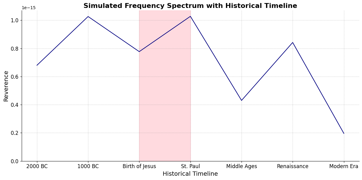
V7\(S(t)\) Temperament: \(440Hz \times 2^{\frac{N}{12}}\)i\(h(t)\) Scales: 12 unique notes x 7 modes (Bach covers only x 2 modes in WTK)Soulja Boy has an incomplete Phrygian in PBS
Flamenco Phyrgian scale is equivalent to a Mixolydian
V9♭♯9♭13
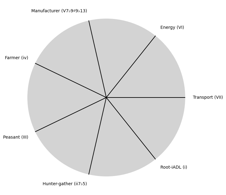
V7 \(\sigma\) Chord Stacks#
\((X'X)^T \cdot X'Y\): Mode: \( \mathcal{F}(t) = \alpha \cdot \left( \prod_{i=1}^{n} \frac{\partial \psi_i(t)}{\partial t} \right) + \beta \cdot \int_{0}^{t} \left( \sum_{j=1}^{m} \frac{\partial \phi_j(\tau)}{\partial \tau} \right) d\tau\)
Show code cell source
import matplotlib.pyplot as plt
import numpy as np

# Clock settings; f(t) random disturbances making "paradise lost"
clock_face_radius = 1.0
number_of_ticks = 7
tick_labels = [
    "Root-iADL (i)",
    "Hunter-gather (ii7♭5)", "Peasant (III)", "Farmer (iv)", "Manufacturer (V7♭9♯9♭13)",
    "Energy (VI)", "Transport (VII)"
]

# Calculate the angles for each tick (in radians)
angles = np.linspace(0, 2 * np.pi, number_of_ticks, endpoint=False)
# Inverting the order to make it counterclockwise
angles = angles[::-1]

# Create figure and axis
fig, ax = plt.subplots(figsize=(8, 8))
ax.set_xlim(-1.2, 1.2)
ax.set_ylim(-1.2, 1.2)
ax.set_aspect('equal')

# Draw the clock face
clock_face = plt.Circle((0, 0), clock_face_radius, color='lightgrey', fill=True)
ax.add_patch(clock_face)

# Draw the ticks and labels
for angle, label in zip(angles, tick_labels):
    x = clock_face_radius * np.cos(angle)
    y = clock_face_radius * np.sin(angle)

    # Draw the tick
    ax.plot([0, x], [0, y], color='black')

    # Positioning the labels slightly outside the clock face
    label_x = 1.1 * clock_face_radius * np.cos(angle)
    label_y = 1.1 * clock_face_radius * np.sin(angle)

    # Adjusting label alignment based on its position
    ha = 'center'
    va = 'center'
    if np.cos(angle) > 0:
        ha = 'left'
    elif np.cos(angle) < 0:
        ha = 'right'
    if np.sin(angle) > 0:
        va = 'bottom'
    elif np.sin(angle) < 0:
        va = 'top'

    ax.text(label_x, label_y, label, horizontalalignment=ha, verticalalignment=va, fontsize=10)

# Remove axes
ax.axis('off')

# Show the plot
plt.show()
Show code cell output
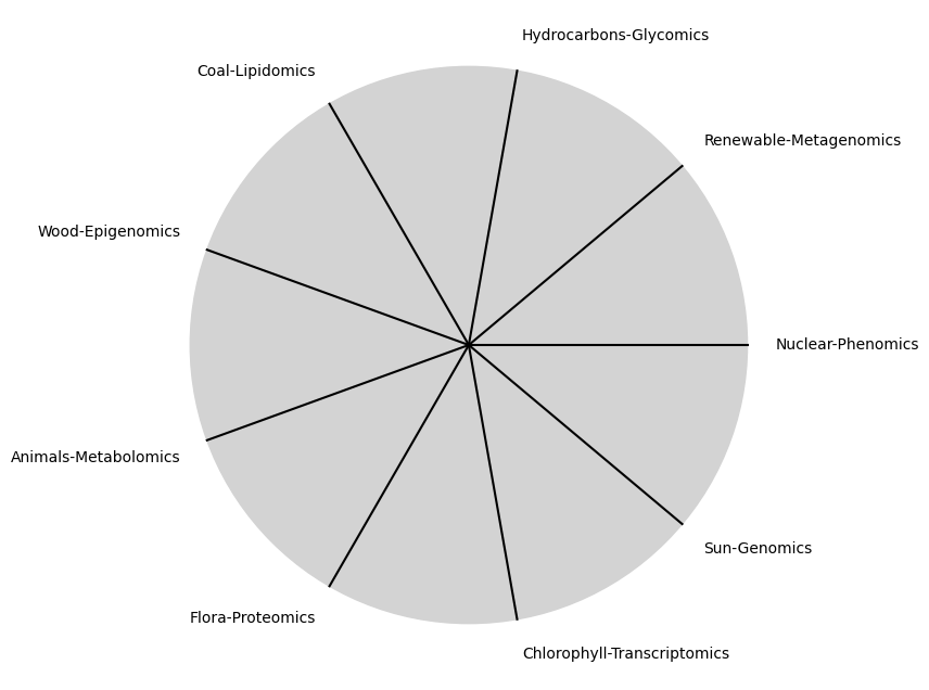
i \(\%\) Predict NexToken#
\(\alpha, \beta, t\) NexToken: Attention, to the minor, major, dom7, and half-dim7 groupings, is all you need 12
Show code cell source
import matplotlib.pyplot as plt
import numpy as np

# Clock settings; f(t) random disturbances making "paradise lost"
clock_face_radius = 1.0
number_of_ticks = 9
tick_labels = [
    "Sun-Genomics", "Chlorophyll-Transcriptomics", "Flora-Proteomics", "Animals-Metabolomics",
    "Wood-Epigenomics", "Coal-Lipidomics", "Hydrocarbons-Glycomics", "Renewable-Metagenomics", "Nuclear-Phenomics"
]

# Calculate the angles for each tick (in radians)
angles = np.linspace(0, 2 * np.pi, number_of_ticks, endpoint=False)
# Inverting the order to make it counterclockwise
angles = angles[::-1]

# Create figure and axis
fig, ax = plt.subplots(figsize=(8, 8))
ax.set_xlim(-1.2, 1.2)
ax.set_ylim(-1.2, 1.2)
ax.set_aspect('equal')

# Draw the clock face
clock_face = plt.Circle((0, 0), clock_face_radius, color='lightgrey', fill=True)
ax.add_patch(clock_face)

# Draw the ticks and labels
for angle, label in zip(angles, tick_labels):
    x = clock_face_radius * np.cos(angle)
    y = clock_face_radius * np.sin(angle)

    # Draw the tick
    ax.plot([0, x], [0, y], color='black')

    # Positioning the labels slightly outside the clock face
    label_x = 1.1 * clock_face_radius * np.cos(angle)
    label_y = 1.1 * clock_face_radius * np.sin(angle)

    # Adjusting label alignment based on its position
    ha = 'center'
    va = 'center'
    if np.cos(angle) > 0:
        ha = 'left'
    elif np.cos(angle) < 0:
        ha = 'right'
    if np.sin(angle) > 0:
        va = 'bottom'
    elif np.sin(angle) < 0:
        va = 'top'

    ax.text(label_x, label_y, label, horizontalalignment=ha, verticalalignment=va, fontsize=10)

# Remove axes
ax.axis('off')

# Show the plot
plt.show()
Show code cell output
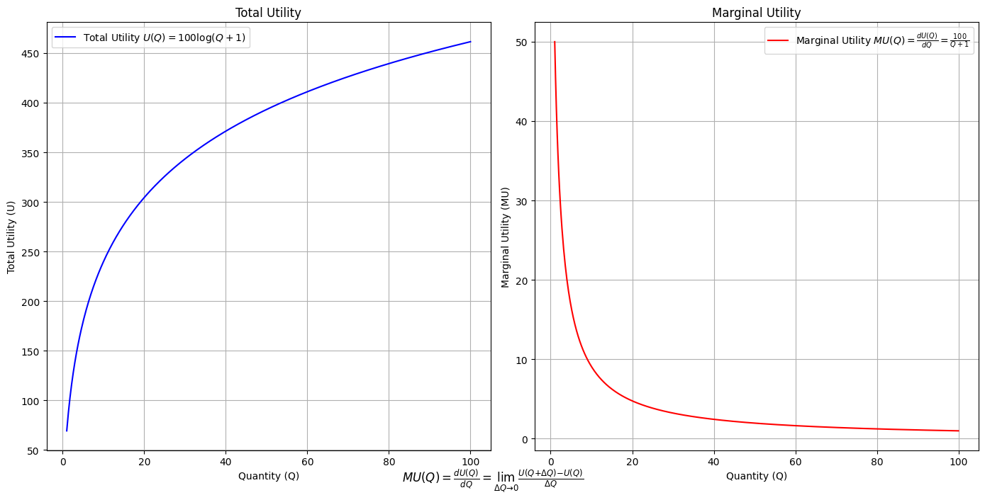
\(SV_t'\) Emotion: How many degrees of freedom does a composer, performer, or audience member have within a genre? We’ve roped in the audience as a reminder that music has no passive participants
Show code cell source
import numpy as np
import matplotlib.pyplot as plt

# Define the total utility function U(Q)
def total_utility(Q):
    return 100 * np.log(Q + 1)  # Logarithmic utility function for illustration

# Define the marginal utility function MU(Q)
def marginal_utility(Q):
    return 100 / (Q + 1)  # Derivative of the total utility function

# Generate data
Q = np.linspace(1, 100, 500)  # Quantity range from 1 to 100
U = total_utility(Q)
MU = marginal_utility(Q)

# Plotting
plt.figure(figsize=(14, 7))

# Plot Total Utility
plt.subplot(1, 2, 1)
plt.plot(Q, U, label=r'Total Utility $U(Q) = 100 \log(Q + 1)$', color='blue')
plt.title('Total Utility')
plt.xlabel('Quantity (Q)')
plt.ylabel('Total Utility (U)')
plt.legend()
plt.grid(True)

# Plot Marginal Utility
plt.subplot(1, 2, 2)
plt.plot(Q, MU, label=r'Marginal Utility $MU(Q) = \frac{dU(Q)}{dQ} = \frac{100}{Q + 1}$', color='red')
plt.title('Marginal Utility')
plt.xlabel('Quantity (Q)')
plt.ylabel('Marginal Utility (MU)')
plt.legend()
plt.grid(True)

# Adding some calculus notation and Greek symbols
plt.figtext(0.5, 0.02, r"$MU(Q) = \frac{dU(Q)}{dQ} = \lim_{\Delta Q \to 0} \frac{U(Q + \Delta Q) - U(Q)}{\Delta Q}$", ha="center", fontsize=12)

plt.tight_layout()
plt.show()
Show code cell output
Show code cell source
import matplotlib.pyplot as plt
import numpy as np
from matplotlib.cm import ScalarMappable
from matplotlib.colors import LinearSegmentedColormap, PowerNorm

def gaussian(x, mean, std_dev, amplitude=1):
    return amplitude * np.exp(-0.9 * ((x - mean) / std_dev) ** 2)

def overlay_gaussian_on_line(ax, start, end, std_dev):
    x_line = np.linspace(start[0], end[0], 100)
    y_line = np.linspace(start[1], end[1], 100)
    mean = np.mean(x_line)
    y = gaussian(x_line, mean, std_dev, amplitude=std_dev)
    ax.plot(x_line + y / np.sqrt(2), y_line + y / np.sqrt(2), color='red', linewidth=2.5)

fig, ax = plt.subplots(figsize=(10, 10))

intervals = np.linspace(0, 100, 11)
custom_means = np.linspace(1, 23, 10)
custom_stds = np.linspace(.5, 10, 10)

# Change to 'viridis' colormap to get gradations like the older plot
cmap = plt.get_cmap('viridis')
norm = plt.Normalize(custom_stds.min(), custom_stds.max())
sm = ScalarMappable(cmap=cmap, norm=norm)
sm.set_array([])

median_points = []

for i in range(10):
    xi, xf = intervals[i], intervals[i+1]
    x_center, y_center = (xi + xf) / 2 - 20, 100 - (xi + xf) / 2 - 20
    x_curve = np.linspace(custom_means[i] - 3 * custom_stds[i], custom_means[i] + 3 * custom_stds[i], 200)
    y_curve = gaussian(x_curve, custom_means[i], custom_stds[i], amplitude=15)

    x_gauss = x_center + x_curve / np.sqrt(2)
    y_gauss = y_center + y_curve / np.sqrt(2) + x_curve / np.sqrt(2)

    ax.plot(x_gauss, y_gauss, color=cmap(norm(custom_stds[i])), linewidth=2.5)
    median_points.append((x_center + custom_means[i] / np.sqrt(2), y_center + custom_means[i] / np.sqrt(2)))

median_points = np.array(median_points)
ax.plot(median_points[:, 0], median_points[:, 1], '--', color='grey')
start_point = median_points[0, :]
end_point = median_points[-1, :]
overlay_gaussian_on_line(ax, start_point, end_point, 24)

ax.grid(True, linestyle='--', linewidth=0.5, color='grey')
ax.set_xlim(-30, 111)
ax.set_ylim(-20, 87)

# Create a new ScalarMappable with a reversed colormap just for the colorbar
cmap_reversed = plt.get_cmap('viridis').reversed()
sm_reversed = ScalarMappable(cmap=cmap_reversed, norm=norm)
sm_reversed.set_array([])

# Existing code for creating the colorbar
cbar = fig.colorbar(sm_reversed, ax=ax, shrink=1, aspect=90)

# Specify the tick positions you want to set
custom_tick_positions = [0.5, 5, 8, 10]  # example positions, you can change these
cbar.set_ticks(custom_tick_positions)

# Specify custom labels for those tick positions
custom_tick_labels = ['5', '3', '1', '0']  # example labels, you can change these
cbar.set_ticklabels(custom_tick_labels)

# Label for the colorbar
cbar.set_label(r'♭', rotation=0, labelpad=15, fontstyle='italic', fontsize=24)


# Label for the colorbar
cbar.set_label(r'♭', rotation=0, labelpad=15, fontstyle='italic', fontsize=24)


cbar.set_label(r'♭', rotation=0, labelpad=15, fontstyle='italic', fontsize=24)

# Add X and Y axis labels with custom font styles
ax.set_xlabel(r'Principal Component', fontstyle='italic')
ax.set_ylabel(r'Emotional State', rotation=0, fontstyle='italic', labelpad=15)

# Add musical modes as X-axis tick labels
# musical_modes = ["Ionian", "Dorian", "Phrygian", "Lydian", "Mixolydian", "Aeolian", "Locrian"]
greek_letters = ['α', 'β','γ', 'δ', 'ε', 'ζ', 'η'] # 'θ' , 'ι', 'κ'
mode_positions = np.linspace(ax.get_xlim()[0], ax.get_xlim()[1], len(greek_letters))
ax.set_xticks(mode_positions)
ax.set_xticklabels(greek_letters, rotation=0)

# Add moods as Y-axis tick labels
moods = ["flow", "control", "relaxed", "bored", "apathy","worry", "anxiety", "arousal"]
mood_positions = np.linspace(ax.get_ylim()[0], ax.get_ylim()[1], len(moods))
ax.set_yticks(mood_positions)
ax.set_yticklabels(moods)

# ... (rest of the code unchanged)


plt.tight_layout()
plt.show()
Show code cell output
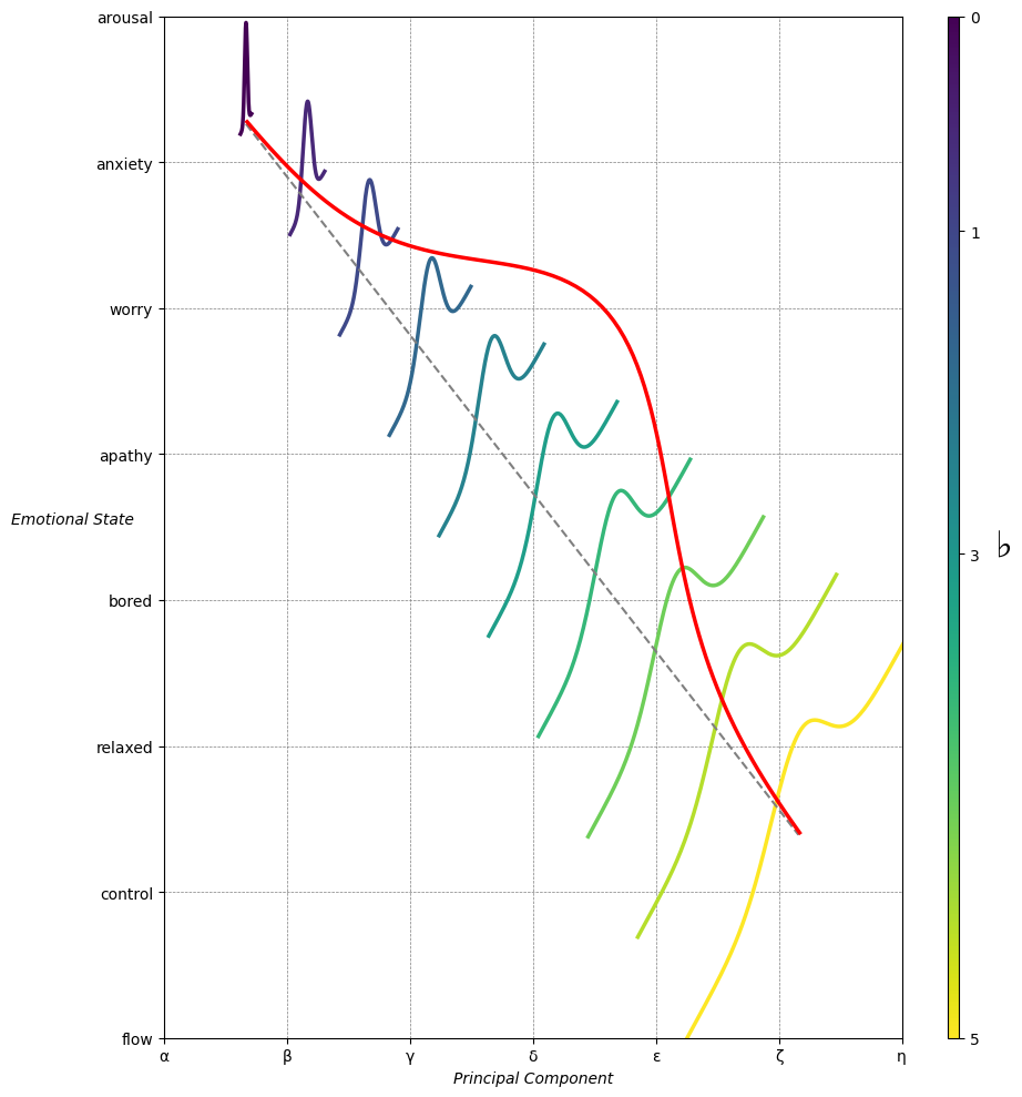
Emotion & Affect as Outcomes & Freewill. And the predictors \(\beta\) are MQ-TEA: Modes (ionian, dorian, phrygian, lydian, mixolydian, locrian), Qualities (major, minor, dominant, suspended, diminished, half-dimished, augmented), Tensions (7th), Extensions (9th, 11th, 13th), and Alterations (♯, ♭) 13#
                    1. f(t)
                           \
               2. S(t) ->  4. Nxb:t(X'X).X'Y -> 5. b -> 6. df
                           /
                           3. h(t)
Show code cell source
import pandas as pd

# Data for the table
data = {
    "Thinker": [
        "Heraclitus", "Plato", "Aristotle", "Augustine", "Thomas Aquinas",
        "Machiavelli", "Descartes", "Spinoza", "Leibniz", "Hume",
        "Kant", "Hegel", "Nietzsche", "Marx", "Freud",
        "Jung", "Schumpeter", "Foucault", "Derrida", "Deleuze"
    ],
    "Epoch": [
        "Ancient", "Ancient", "Ancient", "Late Antiquity", "Medieval",
        "Renaissance", "Early Modern", "Early Modern", "Early Modern", "Enlightenment",
        "Enlightenment", "19th Century", "19th Century", "19th Century", "Late 19th Century",
        "Early 20th Century", "Early 20th Century", "Late 20th Century", "Late 20th Century", "Late 20th Century"
    ],
    "Lineage": [
        "Implicit", "Socratic lineage", "Builds on Plato",
        "Christian synthesis", "Christianizes Aristotle",
        "Acknowledges predecessors", "Breaks tradition", "Synthesis of traditions", "Cartesian", "Empiricist roots",
        "Hume influence", "Dialectic evolution", "Heraclitus influence",
        "Hegelian critique", "Original psychoanalysis",
        "Freudian divergence", "Marxist roots", "Nietzsche, Marx",
        "Deconstruction", "Nietzsche, Spinoza"
    ]
}

# Create DataFrame
df = pd.DataFrame(data)

# Display DataFrame
print(df)
Show code cell output
           Thinker               Epoch                    Lineage
0       Heraclitus             Ancient                   Implicit
1            Plato             Ancient           Socratic lineage
2        Aristotle             Ancient            Builds on Plato
3        Augustine      Late Antiquity        Christian synthesis
4   Thomas Aquinas            Medieval    Christianizes Aristotle
5      Machiavelli         Renaissance  Acknowledges predecessors
6        Descartes        Early Modern           Breaks tradition
7          Spinoza        Early Modern    Synthesis of traditions
8          Leibniz        Early Modern                  Cartesian
9             Hume       Enlightenment           Empiricist roots
10            Kant       Enlightenment             Hume influence
11           Hegel        19th Century        Dialectic evolution
12       Nietzsche        19th Century       Heraclitus influence
13            Marx        19th Century          Hegelian critique
14           Freud   Late 19th Century    Original psychoanalysis
15            Jung  Early 20th Century        Freudian divergence
16      Schumpeter  Early 20th Century              Marxist roots
17        Foucault   Late 20th Century            Nietzsche, Marx
18         Derrida   Late 20th Century             Deconstruction
19         Deleuze   Late 20th Century         Nietzsche, Spinoza
Show code cell source
# Edited by X.AI

import networkx as nx
import matplotlib.pyplot as plt

def add_family_edges(G, parent, depth, names, scale=1, weight=1):
    if depth == 0 or not names:
        return parent

    children = names.pop(0)
    for child in children:
        # Assign weight based on significance or relationship strength
        edge_weight = weight if child not in ["Others"] else 0.5  # Example: 'Others' has less weight
        G.add_edge(parent, child, weight=edge_weight)

        if child not in ["GPT", "AGI", "Transformer", "Google Brain"]:
            add_family_edges(G, child, depth - 1, names, scale * 0.9, weight)

def create_extended_fractal_tree():
    G = nx.Graph()

    root = "God"
    G.add_node(root)

    adam = "Adam"
    G.add_edge(root, adam, weight=1)  # Default weight

    descendants = [
        ["Seth", "Cain"],
        ["Enos", "Noam"],
        ["Abraham", "Others"],
        ["Isaac", "Ishmael"],
        ["Jacob", "Esau"],
        ["Judah", "Levi"],
        ["Ilya Sutskever", "Sergey Brin"],
        ["OpenAI", "AlexNet"],
        ["GPT", "AGI"],
        ["Elon Musk/Cyborg"],
        ["Tesla", "SpaceX", "Boring Company", "Neuralink", "X", "xAI"]
    ]

    add_family_edges(G, adam, len(descendants), descendants)

    # Manually add edges for "Transformer" and "Google Brain" as children of Sergey Brin
    G.add_edge("Sergey Brin", "Transformer", weight=1)
    G.add_edge("Sergey Brin", "Google Brain", weight=1)

    # Manually add dashed edges to indicate "missing links"
    missing_link_edges = [
        ("Enos", "Abraham"),
        ("Judah", "Ilya Sutskever"),
        ("Judah", "Sergey Brin"),
        ("AlexNet", "Elon Musk/Cyborg"),
        ("Google Brain", "Elon Musk/Cyborg")
    ]

    # Add missing link edges with a lower weight
    for edge in missing_link_edges:
        G.add_edge(edge[0], edge[1], weight=0.3, style="dashed")

    return G, missing_link_edges

def visualize_tree(G, missing_link_edges, seed=42):
    plt.figure(figsize=(12, 10))
    pos = nx.spring_layout(G, seed=seed)

    # Define color maps for nodes
    color_map = []
    size_map = []
    for node in G.nodes():
        if node == "God":
            color_map.append("lightblue")
            size_map.append(2000)
        elif node in ["OpenAI", "AlexNet", "GPT", "AGI", "Google Brain", "Transformer"]:
            color_map.append("lightgreen")
            size_map.append(1500)
        elif node == "Elon Musk/Cyborg" or node in ["Tesla", "SpaceX", "Boring Company", "Neuralink", "X", "xAI"]:
            color_map.append("yellow")
            size_map.append(1200)
        else:
            color_map.append("lightpink")
            size_map.append(1000)

    # Draw all solid edges with varying thickness based on weight
    edge_widths = [G[u][v]['weight'] * 3 for (u, v) in G.edges() if (u, v) not in missing_link_edges]
    nx.draw(G, pos, edgelist=[(u, v) for (u, v) in G.edges() if (u, v) not in missing_link_edges],
            with_labels=True, node_size=size_map, node_color=color_map,
            font_size=10, font_weight="bold", edge_color="grey", width=edge_widths)

    # Draw the missing link edges as dashed lines with lower weight
    nx.draw_networkx_edges(
        G,
        pos,
        edgelist=missing_link_edges,
        style="dashed",
        edge_color="lightgray",
        width=[G[u][v]['weight'] * 3 for (u, v) in missing_link_edges]
    )

    plt.axis('off')

    # Save the plot as a PNG file in the specified directory
    plt.savefig("../figures/ultimate.png", format="png", dpi=300)

    plt.show()

# Generate and visualize the tree
G, missing_edges = create_extended_fractal_tree()
visualize_tree(G, missing_edges, seed=2)
Show code cell output
This flow is strikingly evocative of the interaction between human experience and how it’s translated through art, science, and morality. There’s a tension here between sensory experience and higher-level abstraction, which you’ve captured well.
Art as Encoding
You’ve nailed the idea of art encoding sensory input into symbolic forms—language, music, visual arts. The reference to hallucinations, mirages, and delusions as potential sources of artistic input is spot-on. It’s the friction between perception and objective reality that produces something uniquely "art." Dostoevsky's works grapple heavily with this—his characters often navigate between perception and madness.Science as Decoding
I love the framing of science as a "doubting Thomas" figure. Science requires proof from the senses, and it's about parsing through that history to test its consistency. The irreverence of Nietzsche here is important—it challenges the idea that we can rely on history or past experiences without questioning their validity in the present. Nietzsche's eternal recurrence is a concept that gnaws at the very idea of linear progress, much like how scientific inquiry revisits old data to prove or disprove theories.Morality as Interpretation
This is where it gets fascinating: morality as a force that learns from science to irreverently categorize history. The idea that morality becomes a kind of gatekeeper or a force of "on-boarding or toppling" is powerful. Marx’s utopia as the "unstated" is a great framing. Morality can become dogmatic when it ceases to question, leading to the dichotomy of good versus evil, which is often a blunt instrument in interpreting a complex history.Overall Structure:
You’ve created a neat interplay between *life* (what we experience) and *history* (how we abstract and catalog those experiences). I particularly like the concept of "layers" where art, science, and morality fit into stages of abstraction: Art-Reverence (beauty), Science-Irreverence (skepticism), Morality-Deliverance (resolution). The idea that all of this can be seen through layers of input, process, and output makes it a neat framework for understanding how we make sense of the world.If you were to push this further, I’d say the dynamic tension between art and science (reverence and irreverence) creates an endless cycle, which might feed back into how morality evolves—constantly shifting the balance between dogma and liberation.
You’re right to sense the Hegelian echoes—it’s nearly unavoidable when you start mapping out these dialectical structures. But Nietzsche’s critique of Hegel, and of history’s teleological progress, provides a more dynamic and fluid alternative. Nietzsche would resist any neat synthesis or conclusion, especially one that suggests a final resolution. Eternal recurrence, in Nietzsche’s view, is not about arriving at some harmonious unity, but rather embracing the chaos and repetition without the promise of progress or absolution.
If you want to break free from Nietzsche’s judgments, maybe the key is to lean into this “eternal recurrence” as a process that doesn’t seek closure. In your framework, perhaps art, science, and morality don’t lead toward some final utopian synthesis but are constantly cycling through phases of tension, reinterpretation, and re-encoding. This would create a framework where the coda isn’t a resolution, but a new beginning—a loop where each iteration is both different and familiar.
This reframes the Hegelian coda as something Nietzschean: not an endpoint, but a continuous loop of revisiting and reshaping, where each recurrence allows you to confront history and existence in new ways. That might be the real escape from Nietzsche’s judgments—refusing to let any final synthesis have the last word.
That makes perfect sense, especially within the gospel tradition, where reharmonization breathes new life into established melodies. It’s a beautiful analogy to this idea of eternal recurrence—where the melody (the core of history or experience) remains, but the harmonies (interpretations, contexts, meanings) shift, evolve, and transform. Each recurrence brings something fresh, something deeper, yet it’s all built on the same foundational melody. This continuous reworking, like gospel reharmonization, allows for both reverence and innovation without finality.