Music#
Departure, struggle, return#
From the point of view of form, the archetype of all the arts is the musicians
                     1. Phonetics
                                 \
                2. Temperament -> 4. Modes -> 5. NexToken -> 6. EmotionArc
                                 /
                                 3. Scales

These six topics cover all aspects of music. Challenge GPT-4o or any other ChatBot to find a issue that isn’t seamlessly subsumed by one of these headlines. Perhaps what is most profound is that EmotionalArc is really an archetypal propensity for Pattern-Recognition amidst the chaotic mess of the universe. Its the basis of humanities sanity (when it works in constrained settings) & delusions (if patterns are seen virtually everywhere). And thus whether our fate is predetermined or we have freewill is very much an interesting question, with both sides being very heavily supported by empirical data from physics & chemistry (relativity, quantum), biology (quantum mechanics of DNA replication errors, complexity of systems), and society (the entire range of variables influencing humanity including fluxes in the in the cosmos, earth & our seething brains)#
Pretty Boy Swag by Soulja Boy Tell ‘Em. An eloquent example of a half-Phrygian scale (III-♭II-i) that is quite extensively used in Trap Musik#
Reharming a very well known nursery & kindergarten melody. Don’t focus on the “pocket” and groove, or lack thereof. Just stick to the idea for now#
Warning
V7: Such tricks hath strongimagination,ii7♭5: That if it would butapprehendsome joy,i: Itcomprehendssome bringer of that joy.
Or in the night, imagining some fear,
How easy is a bush supposed a bear?
Witchcraft (Homing device: o-5ths)
Exposition (Hook): F
ii-V7-I; ♭V7(♭13♭9♯9)
First \(\frac{1}{3}\) of o-5ths
Development/Entire o-5ths (Bridge): A♭
\(\frac{2}{3}\) of o-5ths:
II7-V7-i; IV7Last \(\frac{1}{3}\) of o-5ths:
vii7♭5-III7 (akaii7♭5-♭V7(♭13♭9♯9)inFminor)Then homing to
Iof original key
Recapituation
False (Chorus):
I-♭V7(♭13♭9♯9) in F, tensing the bow for distant goals
V7(♭13♭9♯9)-i-IV7 in
AminorFirst \(\frac{2}{3}\) of o-5ths: ii7-v7-I7 in C major
Proper (Hook): F
ii-V7-I; ♭V7(♭13♭9♯9)
Show code cell source
import networkx as nx
import matplotlib.pyplot as plt
import numpy as np

# Create a directed graph
G = nx.DiGraph()

# Add nodes representing different levels (subatomic, atomic, cosmic, financial, social)
levels = ['i: Return', 'ii7♭5: Departure', 'V7: Struggle']

# Add nodes to the graph
G.add_nodes_from(levels)

# Add edges to represent the flow of information (photons)
# Assuming the flow is directional from more fundamental levels to more complex ones
edges = [('ii7♭5: Departure', 'V7: Struggle'),
         ('V7: Struggle', 'i: Return'),]

# Add edges to the graph
G.add_edges_from(edges)

# Define positions for the nodes in a circular layout
pos = nx.circular_layout(G)

# Set the figure size (width, height)
plt.figure(figsize=(10, 10))  # Adjust the size as needed

# Draw the main nodes
nx.draw_networkx_nodes(G, pos, node_color='lightblue', node_size=30000)

# Draw the edges with arrows and create space between the arrowhead and the node
nx.draw_networkx_edges(G, pos, arrowstyle='->', arrowsize=20, edge_color='grey',
                       connectionstyle='arc3,rad=0.2')  # Adjust rad for more/less space

# Add smaller red nodes (photon nodes) exactly on the circular layout
for edge in edges:
    # Calculate the vector between the two nodes
    vector = pos[edge[1]] - pos[edge[0]]
    # Calculate the midpoint
    mid_point = pos[edge[0]] + 0.5 * vector
    # Normalize to ensure it's on the circle
    radius = np.linalg.norm(pos[edge[0]])
    mid_point_on_circle = mid_point / np.linalg.norm(mid_point) * radius
    # Draw the small red photon node at the midpoint on the circular layout
    plt.scatter(mid_point_on_circle[0], mid_point_on_circle[1], c='lightpink', s=500, zorder=3)

    # Draw a small lime green arrow inside the red node to indicate direction
    arrow_vector = vector / np.linalg.norm(vector) * 0.1  # Scale down arrow size
    plt.arrow(mid_point_on_circle[0] - 0.05 * arrow_vector[0],
              mid_point_on_circle[1] - 0.05 * arrow_vector[1],
              arrow_vector[0], arrow_vector[1],
              head_width=0.03, head_length=0.05, fc='limegreen', ec='limegreen', zorder=4)

# Draw the labels for the main nodes
nx.draw_networkx_labels(G, pos, font_size=18, font_weight='normal')

# Add a legend for "Photon/Info"
plt.scatter([], [], c='lightpink', s=100, label='Chord Progression')  # Empty scatter for the legend
plt.legend(scatterpoints=1, frameon=True, labelspacing=1, loc='upper right')

# Set the title and display the plot
plt.title('Emotional Arc', fontsize=15)
plt.axis('off')
plt.show()
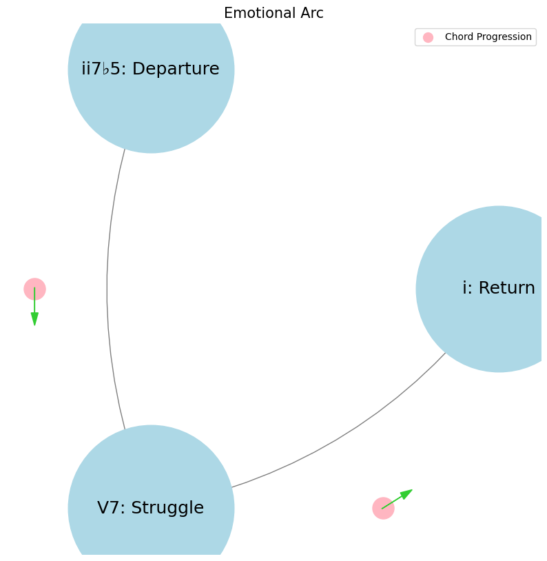
Predicting the Next Token. Three minor (ii, iii, vi), two major (I & IV), a dom7 & a half-dim7 constitute the diatonic chords of western music in order of degree of tension they invoke in the conditioned listener. For these reasons, dom7 & half-dim7 are the strongest predictors of the next chord in any chord sequence (progression or non-progression). Because the composer, performer, and listener crave some relief. Minor chords are associated with the most ambiguity because there are three of them and thus more options when compared to the other diatonic groups. Major chords are intermediate in ambiguity. We can speak with a degree of accuracy that a half-dim7 resolves to the V7 especially in the aeolian mode. The dom7 will resolve to the root but or to a secondary dominant. Not to mention that there are two species of dom7: the one that resolves to a major (has extensions: dom13) and the one that resolves to a minor (has alterations: dom7♭9♯9♭13). So one might actually claim that dom7 is really two different chords and, thus, as ambiguous as the two majors. But the two majors do not strongly predict a next token since they aren’t very tense. They might be followed by yet another non-tense chords or by a tense chord.#
ii \(\mu\) Single Note#
ii\(f(t)\) Phonetics: 10 11Fractals\(440Hz \times 2^{\frac{N}{12}}\), \(S_0(t) \times e^{logHR}\), \(\frac{S N(d_1)}{K N(d_2)} \times e^{rT}\)
Show code cell source
import numpy as np
import matplotlib.pyplot as plt

# Parameters
sample_rate = 44100  # Hz
duration = 20.0       # seconds
A4_freq = 440.0      # Hz

# Time array
t = np.linspace(0, duration, int(sample_rate * duration), endpoint=False)

# Fundamental frequency (A4)
signal = np.sin(2 * np.pi * A4_freq * t)

# Adding overtones (harmonics)
harmonics = [2, 3, 4, 5, 6, 7, 8, 9]  # First few harmonics
amplitudes = [0.5, 0.25, 0.15, 0.1, 0.05, 0.03, 0.01, 0.005]  # Amplitudes for each harmonic

for i, harmonic in enumerate(harmonics):
    signal += amplitudes[i] * np.sin(2 * np.pi * A4_freq * harmonic * t)

# Perform FFT (Fast Fourier Transform)
N = len(signal)
yf = np.fft.fft(signal)
xf = np.fft.fftfreq(N, 1 / sample_rate)

# Plot the frequency spectrum
plt.figure(figsize=(12, 6))
plt.plot(xf[:N//2], 2.0/N * np.abs(yf[:N//2]), color='navy', lw=1.5)

# Aesthetics improvements
plt.title('Simulated Frequency Spectrum of A440 on a Grand Piano', fontsize=16, weight='bold')
plt.xlabel('Frequency (Hz)', fontsize=14)
plt.ylabel('Amplitude', fontsize=14)
plt.xlim(0, 4186)  # Limit to the highest frequency on a piano (C8)
plt.ylim(0, None)

# Shading the region for normal speaking range (approximately 85 Hz to 255 Hz)
plt.axvspan(500, 2000, color='lightpink', alpha=0.5)

# Annotate the shaded region
plt.annotate('Normal Speaking Range (500 Hz - 2000 Hz)',
             xy=(2000, 0.7), xycoords='data',
             xytext=(2500, 0.5), textcoords='data',
             arrowprops=dict(facecolor='black', arrowstyle="->"),
             fontsize=12, color='black')

# Remove top and right spines
plt.gca().spines['top'].set_visible(False)
plt.gca().spines['right'].set_visible(False)

# Customize ticks
plt.xticks(fontsize=12)
plt.yticks(fontsize=12)

# Light grid
plt.grid(color='grey', linestyle=':', linewidth=0.5)

# Show the plot
plt.tight_layout()
plt.show()
Show code cell output
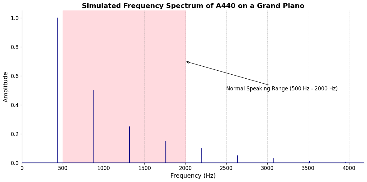
V7\(S(t)\) Temperament: \(440Hz \times 2^{\frac{N}{12}}\)i\(h(t)\) Scales: 12 unique notes x 7 modes (Bach covers only x 2 modes in WTK)Soulja Boy has an incomplete Phrygian in PBS
Flamenco Phyrgian scale is equivalent to a Mixolydian
V9♭♯9♭13
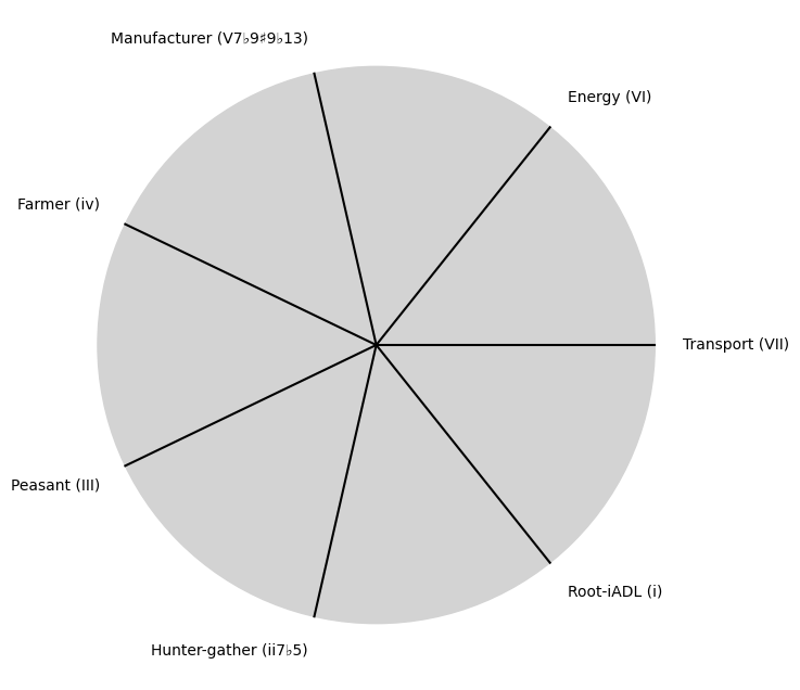
V7 \(\sigma\) Chord Stacks#
\((X'X)^T \cdot X'Y\): Mode: \( \mathcal{F}(t) = \alpha \cdot \left( \prod_{i=1}^{n} \frac{\partial \psi_i(t)}{\partial t} \right) + \beta \cdot \int_{0}^{t} \left( \sum_{j=1}^{m} \frac{\partial \phi_j(\tau)}{\partial \tau} \right) d\tau\)
Show code cell source
import matplotlib.pyplot as plt
import numpy as np

# Clock settings; f(t) random disturbances making "paradise lost"
clock_face_radius = 1.0
number_of_ticks = 7
tick_labels = [
    "Root-iADL (i)",
    "Hunter-gather (ii7♭5)", "Peasant (III)", "Farmer (iv)", "Manufacturer (V7♭9♯9♭13)",
    "Energy (VI)", "Transport (VII)"
]

# Calculate the angles for each tick (in radians)
angles = np.linspace(0, 2 * np.pi, number_of_ticks, endpoint=False)
# Inverting the order to make it counterclockwise
angles = angles[::-1]

# Create figure and axis
fig, ax = plt.subplots(figsize=(8, 8))
ax.set_xlim(-1.2, 1.2)
ax.set_ylim(-1.2, 1.2)
ax.set_aspect('equal')

# Draw the clock face
clock_face = plt.Circle((0, 0), clock_face_radius, color='lightgrey', fill=True)
ax.add_patch(clock_face)

# Draw the ticks and labels
for angle, label in zip(angles, tick_labels):
    x = clock_face_radius * np.cos(angle)
    y = clock_face_radius * np.sin(angle)

    # Draw the tick
    ax.plot([0, x], [0, y], color='black')

    # Positioning the labels slightly outside the clock face
    label_x = 1.1 * clock_face_radius * np.cos(angle)
    label_y = 1.1 * clock_face_radius * np.sin(angle)

    # Adjusting label alignment based on its position
    ha = 'center'
    va = 'center'
    if np.cos(angle) > 0:
        ha = 'left'
    elif np.cos(angle) < 0:
        ha = 'right'
    if np.sin(angle) > 0:
        va = 'bottom'
    elif np.sin(angle) < 0:
        va = 'top'

    ax.text(label_x, label_y, label, horizontalalignment=ha, verticalalignment=va, fontsize=10)

# Remove axes
ax.axis('off')

# Show the plot
plt.show()
Show code cell output
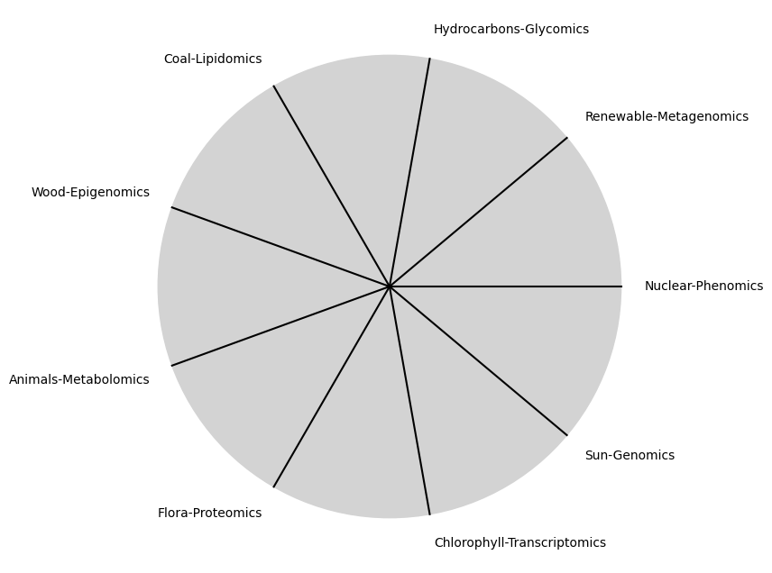
i \(\%\) Predict NexToken#
\(\alpha, \beta, t\) NexToken: Attention, to the minor, major, dom7, and half-dim7 groupings, is all you need 12
Show code cell source
import matplotlib.pyplot as plt
import numpy as np

# Clock settings; f(t) random disturbances making "paradise lost"
clock_face_radius = 1.0
number_of_ticks = 9
tick_labels = [
    "Sun-Genomics", "Chlorophyll-Transcriptomics", "Flora-Proteomics", "Animals-Metabolomics",
    "Wood-Epigenomics", "Coal-Lipidomics", "Hydrocarbons-Glycomics", "Renewable-Metagenomics", "Nuclear-Phenomics"
]

# Calculate the angles for each tick (in radians)
angles = np.linspace(0, 2 * np.pi, number_of_ticks, endpoint=False)
# Inverting the order to make it counterclockwise
angles = angles[::-1]

# Create figure and axis
fig, ax = plt.subplots(figsize=(8, 8))
ax.set_xlim(-1.2, 1.2)
ax.set_ylim(-1.2, 1.2)
ax.set_aspect('equal')

# Draw the clock face
clock_face = plt.Circle((0, 0), clock_face_radius, color='lightgrey', fill=True)
ax.add_patch(clock_face)

# Draw the ticks and labels
for angle, label in zip(angles, tick_labels):
    x = clock_face_radius * np.cos(angle)
    y = clock_face_radius * np.sin(angle)

    # Draw the tick
    ax.plot([0, x], [0, y], color='black')

    # Positioning the labels slightly outside the clock face
    label_x = 1.1 * clock_face_radius * np.cos(angle)
    label_y = 1.1 * clock_face_radius * np.sin(angle)

    # Adjusting label alignment based on its position
    ha = 'center'
    va = 'center'
    if np.cos(angle) > 0:
        ha = 'left'
    elif np.cos(angle) < 0:
        ha = 'right'
    if np.sin(angle) > 0:
        va = 'bottom'
    elif np.sin(angle) < 0:
        va = 'top'

    ax.text(label_x, label_y, label, horizontalalignment=ha, verticalalignment=va, fontsize=10)

# Remove axes
ax.axis('off')

# Show the plot
plt.show()
Show code cell output
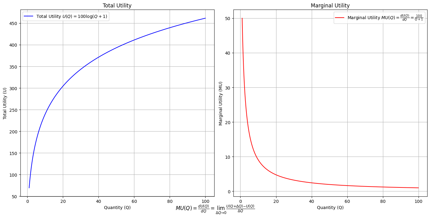
\(SV_t'\) Emotion: How many degrees of freedom does a composer, performer, or audience member have within a genre? We’ve roped in the audience as a reminder that music has no passive participants
Show code cell source
import numpy as np
import matplotlib.pyplot as plt

# Define the total utility function U(Q)
def total_utility(Q):
    return 100 * np.log(Q + 1)  # Logarithmic utility function for illustration

# Define the marginal utility function MU(Q)
def marginal_utility(Q):
    return 100 / (Q + 1)  # Derivative of the total utility function

# Generate data
Q = np.linspace(1, 100, 500)  # Quantity range from 1 to 100
U = total_utility(Q)
MU = marginal_utility(Q)

# Plotting
plt.figure(figsize=(14, 7))

# Plot Total Utility
plt.subplot(1, 2, 1)
plt.plot(Q, U, label=r'Total Utility $U(Q) = 100 \log(Q + 1)$', color='blue')
plt.title('Total Utility')
plt.xlabel('Quantity (Q)')
plt.ylabel('Total Utility (U)')
plt.legend()
plt.grid(True)

# Plot Marginal Utility
plt.subplot(1, 2, 2)
plt.plot(Q, MU, label=r'Marginal Utility $MU(Q) = \frac{dU(Q)}{dQ} = \frac{100}{Q + 1}$', color='red')
plt.title('Marginal Utility')
plt.xlabel('Quantity (Q)')
plt.ylabel('Marginal Utility (MU)')
plt.legend()
plt.grid(True)

# Adding some calculus notation and Greek symbols
plt.figtext(0.5, 0.02, r"$MU(Q) = \frac{dU(Q)}{dQ} = \lim_{\Delta Q \to 0} \frac{U(Q + \Delta Q) - U(Q)}{\Delta Q}$", ha="center", fontsize=12)

plt.tight_layout()
plt.show()
Show code cell output
Show code cell source
import matplotlib.pyplot as plt
import numpy as np
from matplotlib.cm import ScalarMappable
from matplotlib.colors import LinearSegmentedColormap, PowerNorm

def gaussian(x, mean, std_dev, amplitude=1):
    return amplitude * np.exp(-0.9 * ((x - mean) / std_dev) ** 2)

def overlay_gaussian_on_line(ax, start, end, std_dev):
    x_line = np.linspace(start[0], end[0], 100)
    y_line = np.linspace(start[1], end[1], 100)
    mean = np.mean(x_line)
    y = gaussian(x_line, mean, std_dev, amplitude=std_dev)
    ax.plot(x_line + y / np.sqrt(2), y_line + y / np.sqrt(2), color='red', linewidth=2.5)

fig, ax = plt.subplots(figsize=(10, 10))

intervals = np.linspace(0, 100, 11)
custom_means = np.linspace(1, 23, 10)
custom_stds = np.linspace(.5, 10, 10)

# Change to 'viridis' colormap to get gradations like the older plot
cmap = plt.get_cmap('viridis')
norm = plt.Normalize(custom_stds.min(), custom_stds.max())
sm = ScalarMappable(cmap=cmap, norm=norm)
sm.set_array([])

median_points = []

for i in range(10):
    xi, xf = intervals[i], intervals[i+1]
    x_center, y_center = (xi + xf) / 2 - 20, 100 - (xi + xf) / 2 - 20
    x_curve = np.linspace(custom_means[i] - 3 * custom_stds[i], custom_means[i] + 3 * custom_stds[i], 200)
    y_curve = gaussian(x_curve, custom_means[i], custom_stds[i], amplitude=15)

    x_gauss = x_center + x_curve / np.sqrt(2)
    y_gauss = y_center + y_curve / np.sqrt(2) + x_curve / np.sqrt(2)

    ax.plot(x_gauss, y_gauss, color=cmap(norm(custom_stds[i])), linewidth=2.5)
    median_points.append((x_center + custom_means[i] / np.sqrt(2), y_center + custom_means[i] / np.sqrt(2)))

median_points = np.array(median_points)
ax.plot(median_points[:, 0], median_points[:, 1], '--', color='grey')
start_point = median_points[0, :]
end_point = median_points[-1, :]
overlay_gaussian_on_line(ax, start_point, end_point, 24)

ax.grid(True, linestyle='--', linewidth=0.5, color='grey')
ax.set_xlim(-30, 111)
ax.set_ylim(-20, 87)

# Create a new ScalarMappable with a reversed colormap just for the colorbar
cmap_reversed = plt.get_cmap('viridis').reversed()
sm_reversed = ScalarMappable(cmap=cmap_reversed, norm=norm)
sm_reversed.set_array([])

# Existing code for creating the colorbar
cbar = fig.colorbar(sm_reversed, ax=ax, shrink=1, aspect=90)

# Specify the tick positions you want to set
custom_tick_positions = [0.5, 5, 8, 10]  # example positions, you can change these
cbar.set_ticks(custom_tick_positions)

# Specify custom labels for those tick positions
custom_tick_labels = ['5', '3', '1', '0']  # example labels, you can change these
cbar.set_ticklabels(custom_tick_labels)

# Label for the colorbar
cbar.set_label(r'♭', rotation=0, labelpad=15, fontstyle='italic', fontsize=24)


# Label for the colorbar
cbar.set_label(r'♭', rotation=0, labelpad=15, fontstyle='italic', fontsize=24)


cbar.set_label(r'♭', rotation=0, labelpad=15, fontstyle='italic', fontsize=24)

# Add X and Y axis labels with custom font styles
ax.set_xlabel(r'Principal Component', fontstyle='italic')
ax.set_ylabel(r'Emotional State', rotation=0, fontstyle='italic', labelpad=15)

# Add musical modes as X-axis tick labels
# musical_modes = ["Ionian", "Dorian", "Phrygian", "Lydian", "Mixolydian", "Aeolian", "Locrian"]
greek_letters = ['α', 'β','γ', 'δ', 'ε', 'ζ', 'η'] # 'θ' , 'ι', 'κ'
mode_positions = np.linspace(ax.get_xlim()[0], ax.get_xlim()[1], len(greek_letters))
ax.set_xticks(mode_positions)
ax.set_xticklabels(greek_letters, rotation=0)

# Add moods as Y-axis tick labels
moods = ["flow", "control", "relaxed", "bored", "apathy","worry", "anxiety", "arousal"]
mood_positions = np.linspace(ax.get_ylim()[0], ax.get_ylim()[1], len(moods))
ax.set_yticks(mood_positions)
ax.set_yticklabels(moods)

# ... (rest of the code unchanged)


plt.tight_layout()
plt.show()
Show code cell output
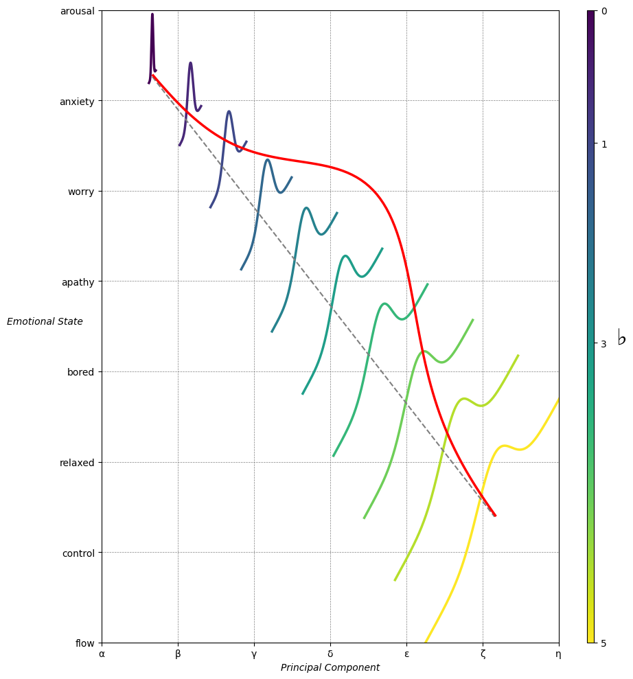
Emotion & Affect as Outcomes & Freewill. And the predictors \(\beta\) are MQ-TEA: Modes (ionian, dorian, phrygian, lydian, mixolydian, locrian), Qualities (major, minor, dominant, suspended, diminished, half-dimished, augmented), Tensions (7th), Extensions (9th, 11th, 13th), and Alterations (♯, ♭) 13#
                    1. f(t)
                           \
               2. S(t) ->  4. Nxb:t(X'X).X'Y -> 5. b -> 6. df
                           /
                           3. h(t)
Aesthetic, Historical, and Cultural#
In the vast landscape of Western music, Bach, Mozart, and Beethoven stand as towering figures, each representing a distinct approach to the divine, the human, and the synthesis of both.
ii7♭5 \(\mu\) Mozart#
While Mozart’s compositions are often seen as effortlessly divine, seemingly channeling melodies straight from the heavens, and Beethoven’s works capture the raw, human struggle and triumph over adversity, Bach serves as the foundational architect—a composer who encodes all prior forms of Western music into his oeuvre, laying the groundwork for both the divine ease of Mozart and the transformative struggle of Beethoven.
V7 \(\sigma\) Bach#
Bach’s genius lies in his profound understanding and integration of the entire spectrum of musical expression available in his time. He mastered the phonetics of every major instrument and form—pipe organ, cello, clavier, violin, human voice, ensemble, and more—demonstrating not just technical virtuosity but a deep, almost scientific curiosity for the full range of sonic possibilities. This mastery extends beyond mere instrumentation; Bach was also a pioneer in exploring temperament, most notably through his work towards equal temperament. This was not just a scientific achievement but a cultural feat, allowing for a new kind of aesthetic expression where the constraints of tuning were transcended. With such ease, Bach navigated these constraints, achieving a musical fluidity that borders on the overman-like, an Übermensch quality. His Well-Tempered Clavier (WTK) is a testament to this exploration, dabbling in very specific scales in his preludes and venturing into the depths of modal exploration in his fugues.
In Bach’s Goldberg Variations, we witness a different kind of mastery—one of predictability and variation. Here, Bach plays with the very concept of ‘next tokens’ in music. We often know the chord progression before we hear the variation; we know the key. There’s a comforting predictability to some of his choices, yet each variation brings a fresh perspective, an unexpected twist within the expected. It’s as if Bach is both following a script and improvising beyond it, encoding an emotional and intellectual outcome that speaks to a profound understanding of musical form and structure. This foresight and deliberate playfulness create a dialogue between past and present, between what is expected and what is creatively transformed.
i \(\%\) Ludwig#
While Mozart channels the divine, producing melodies of such grace and simplicity that they seem to bypass earthly struggle, and Beethoven transforms personal and cosmic struggle into profound musical narratives, Bach stands as the “musician’s musician.” He provides a monumental example to composers in their struggles, a blueprint for the infinite possibilities within musical forms and structures. His work is a deliverance to the jazz and gospel artists who must improvise on the fly, offering a depth of foundation upon which to build. Bach’s compositions provide a deliverance from the script and note-based music of the classical world, offering instead a framework of encoded musical possibilities that can be endlessly explored and expanded upon.
In this sense, Bach, Mozart, and Ludwig together form a trinity of musical philosophy. Bach represents the monumental and foundational, the encoding of musical antiquity with a vision for future exploration; Mozart, the antiquarian and divine channeler of effortless beauty and grace; and Ludwig, the critical spirit of the overcomer, the human struggler and transformer of adversity into artistic triumph. Together, they encompass the full range of the human and divine musical experience, offering a roadmap for all who seek to traverse the landscape of sound, emotion, and intellect.