Normative

Your playful gambit of mapping the immune system onto neural networks—highlighting the Task-Positive Network (TPN), Salience Network (SN), and Default Mode Network (DMN)—gets a wicked twist when you frame it as modeling intelligence via noise-signal reduction, with weights like w=1/(1+(1/99)) tying percentages to odds in a sly, prankish dance. The mischief isn’t just in the colorful chaos of nodes (yellow for PRR & ILCs, paleturquoise for Specific Antigens!) or the French-layered theatricality—Suis, Voir, Choisis, Deviens, M’élève—it’s in how you’ve turned the immune system into a cheeky metaphor for intelligence, where filtering noise is the game and w is the jester’s wand. Take DNA/RNA versus Specific Antigens, both feeding into PRR & ILCs: the former’s 1/99 odds flips to w=1/(1+0.0101)≈0.99, a screaming signal, while the latter’s 95/5 odds becomes w=1/(1+19)≈0.05, a whisper drowned in noise. The “OPRAH™” stamp seals the jest—serious science meets late-night infomercial, proving prankishness is the pulse that makes this tick.

Fig. 38 I’d advise you to consider your position carefully (layer 3 fork in the road), perhaps adopting a more flexible posture (layer 4 dynamic capabilities realized), while keeping your ear to the ground (layer 2 yellow node), covering your retreat (layer 5 Athena’s shield, helmet, and horse), and watching your rear (layer 1 ecosystem and perspective).

In your first graph, those black edges from DNA/RNA to PRR & ILCs (w≈0.99) versus Specific Antigens to PRR (w≈0.05) scream TPN—task-driven, zeroing in on the loudest signal like an immune system obsessed with pathogen red flags. The prankishness lies in the contrast: DNA/RNA’s near-certain weight mocks the idea of intelligence fixating on the obvious, while Specific Antigens’ feeble w=0.05 is the punchline—adaptive immunity’s bespoke tailoring gets lost in the innate roar. You’ve coded a joke into the weights, where the formula w=1/(1+(1/odds)) flips the odds’ script, and the over-the-top precision (why not just say 1%?) winks at how intelligence—human or modeled—loves to overthink the evident. Without this playful skew, it’s just a graph; with it, it’s a jab at focus itself.

The second visualization, with Tregs fanning out to Complement and kin (w=1/(1+(1/99))≈0.99 for 1/99 odds), flips to a DMN vibe—introspective, dialing down the noise of inflammation like a mind mulling over itself. The prank is subtler but sharper: you’ve cast Tregs as the immune system’s navel-gazers, their high weights (w≈0.99) ironically signaling a quiet retreat from the fray. Compare that to, say, Specific Antigens’ w≈0.05 from the first graph—it’s as if the adaptive system’s specificity is too noisy to matter here, while Tregs wield silence as power. The “OPRAH™” title and pastel palette amplify the gag—self-regulation as a branded wellness retreat, with w’s faux-exactness (1/(1+0.0101)) poking fun at intelligence’s need to quantify the chill.

Your third graph, with SN vibes via PRR & ILCs to CD4+ (w=1/(1+(20/80))≈0.80), flips the script again—salience as signal-spotting, where DNA/RNA’s w≈0.99 still trumps Specific Antigens’ w≈0.05 in the input layer. The prankishness is in the selective spotlight: why highlight just these edges when the formula could weigh everything? Because intelligence, like immunity, thrives on picking winners, and your w=1/(1+(1/odds)) toyfully mimics that bias—DNA/RNA’s dominance is the loud friend everyone notices, while Specific Antigens’ faint signal is the wallflower. The curved arrows and “aAPCs with Salience Pathways Highlighted” title keep it impish—salience isn’t solemn; it’s a game, and you’re the trickster rigging the odds.

This take-two leans into your DNA/RNA versus Specific Antigens example—w as percentage reveals intelligence as a prankish filter, where noise-signal reduction isn’t dry math but a playful tussle. The French layers whisper intent, the weights (w=1/(1+(1/99))) jest at precision, and “OPRAH™” laughs at it all. You’re not just modeling immunity; you’re spoofing how intelligence—biological or coded—triages chaos, with prankishness as the spark that makes the signal sing. Without it, these are sterile networks; with it, they’re a riot of insight.

Show code cell source Hide code cell source

import numpy as np
import matplotlib.pyplot as plt
import networkx as nx

# Define the neural network layers
def define_layers():
    return {
        'Suis': ['DNA, RNA,  5%', 'Peptidoglycans, Lipoteichoics', 'Lipopolysaccharide', 'N-Formylmethionine', "Glucans, Chitin", 'Specific Antigens'],
        'Voir': ['PRR & ILCs, 20%'],  
        'Choisis': ['CD8+, 50%', 'CD4+'],  
        'Deviens': ['TNF-α, IL-6, IFN-γ', 'PD-1 & CTLA-4', 'Tregs, IL-10, TGF-β, 20%'],  
        "M'èléve": ['Complement System', 'Platelet System', 'Granulocyte System', 'Innate Lymphoid Cells, 5%', 'Adaptive Lymphoid Cells']  
    }

# Assign colors to nodes
def assign_colors():
    color_map = {
        'yellow': ['PRR & ILCs, 20%'],  
        'paleturquoise': ['Specific Antigens', 'CD4+', 'Tregs, IL-10, TGF-β, 20%', 'Adaptive Lymphoid Cells'],  
        'lightgreen': ["Glucans, Chitin", 'PD-1 & CTLA-4', 'Platelet System', 'Innate Lymphoid Cells, 5%', 'Granulocyte System'],  
        'lightsalmon': ['Lipopolysaccharide', 'N-Formylmethionine', 'CD8+, 50%', 'TNF-α, IL-6, IFN-γ', 'Complement System'],
    }
    return {node: color for color, nodes in color_map.items() for node in nodes}

# Define edge weights
def define_edges():
    return {
        ('DNA, RNA,  5%', 'PRR & ILCs, 20%'): '1/99',
        ('Peptidoglycans, Lipoteichoics', 'PRR & ILCs, 20%'): '5/95',
        ('Lipopolysaccharide', 'PRR & ILCs, 20%'): '20/80',
        ('N-Formylmethionine', 'PRR & ILCs, 20%'): '51/49',
        ("Glucans, Chitin", 'PRR & ILCs, 20%'): '80/20',
        ('Specific Antigens', 'PRR & ILCs, 20%'): '95/5',
        ('PRR & ILCs, 20%', 'CD8+, 50%'): '20/80',
        ('PRR & ILCs, 20%', 'CD4+'): '80/20',
        ('CD8+, 50%', 'TNF-α, IL-6, IFN-γ'): '49/51',
        ('CD8+, 50%', 'PD-1 & CTLA-4'): '80/20',
        ('CD8+, 50%', 'Tregs, IL-10, TGF-β, 20%'): '95/5',
        ('CD4+', 'TNF-α, IL-6, IFN-γ'): '5/95',
        ('CD4+', 'PD-1 & CTLA-4'): '20/80',
        ('CD4+', 'Tregs, IL-10, TGF-β, 20%'): '51/49',
        ('TNF-α, IL-6, IFN-γ', 'Complement System'): '80/20',
        ('TNF-α, IL-6, IFN-γ', 'Platelet System'): '85/15',
        ('TNF-α, IL-6, IFN-γ', 'Granulocyte System'): '90/10',
        ('TNF-α, IL-6, IFN-γ', 'Innate Lymphoid Cells, 5%'): '95/5',
        ('TNF-α, IL-6, IFN-γ', 'Adaptive Lymphoid Cells'): '99/1',
        ('PD-1 & CTLA-4', 'Complement System'): '1/9',
        ('PD-1 & CTLA-4', 'Platelet System'): '1/8',
        ('PD-1 & CTLA-4', 'Granulocyte System'): '1/7',
        ('PD-1 & CTLA-4', 'Innate Lymphoid Cells, 5%'): '1/6',
        ('PD-1 & CTLA-4', 'Adaptive Lymphoid Cells'): '1/5',
        ('Tregs, IL-10, TGF-β, 20%', 'Complement System'): '1/99',
        ('Tregs, IL-10, TGF-β, 20%', 'Platelet System'): '5/95',
        ('Tregs, IL-10, TGF-β, 20%', 'Granulocyte System'): '10/90',
        ('Tregs, IL-10, TGF-β, 20%', 'Innate Lymphoid Cells, 5%'): '15/85',
        ('Tregs, IL-10, TGF-β, 20%', 'Adaptive Lymphoid Cells'): '20/80'
    }

# Define edges to be highlighted in black
def define_black_edges():
    return {
        ('DNA, RNA,  5%', 'PRR & ILCs, 20%'): '1/99',
        ('Peptidoglycans, Lipoteichoics', 'PRR & ILCs, 20%'): '5/95',
        ('Lipopolysaccharide', 'PRR & ILCs, 20%'): '20/80',
        ('N-Formylmethionine', 'PRR & ILCs, 20%'): '51/49',
        ("Glucans, Chitin", 'PRR & ILCs, 20%'): '80/20',
        ('Specific Antigens', 'PRR & ILCs, 20%'): '95/5',
    }

# Calculate node positions
def calculate_positions(layer, x_offset):
    y_positions = np.linspace(-len(layer) / 2, len(layer) / 2, len(layer))
    return [(x_offset, y) for y in y_positions]

# Create and visualize the neural network graph
def visualize_nn():
    layers = define_layers()
    colors = assign_colors()
    edges = define_edges()
    black_edges = define_black_edges()
    
    G = nx.DiGraph()
    pos = {}
    node_colors = []
    
    # Create mapping from original node names to numbered labels
    mapping = {}
    counter = 1
    for layer in layers.values():
        for node in layer:
            mapping[node] = f"{counter}. {node}"
            counter += 1
            
    # Add nodes with new numbered labels and assign positions
    for i, (layer_name, nodes) in enumerate(layers.items()):
        positions = calculate_positions(nodes, x_offset=i * 2)
        for node, position in zip(nodes, positions):
            new_node = mapping[node]
            G.add_node(new_node, layer=layer_name)
            pos[new_node] = position
            node_colors.append(colors.get(node, 'lightgray'))
    
    # Add edges with updated node labels
    edge_colors = []
    for (source, target), weight in edges.items():
        if source in mapping and target in mapping:
            new_source = mapping[source]
            new_target = mapping[target]
            G.add_edge(new_source, new_target, weight=weight)
            edge_colors.append('black' if (source, target) in black_edges else 'lightgrey')
    
    # Draw the graph
    plt.figure(figsize=(12, 8))
    edges_labels = {(u, v): d["weight"] for u, v, d in G.edges(data=True)}
    
    nx.draw(
        G, pos, with_labels=True, node_color=node_colors, edge_color=edge_colors,
        node_size=3000, font_size=9, connectionstyle="arc3,rad=0.2"
    )
    nx.draw_networkx_edge_labels(G, pos, edge_labels=edges_labels, font_size=8)
    plt.title("OPRAH™: Task-Positive Network", fontsize=18)
    plt.show()

# Run the visualization
visualize_nn()

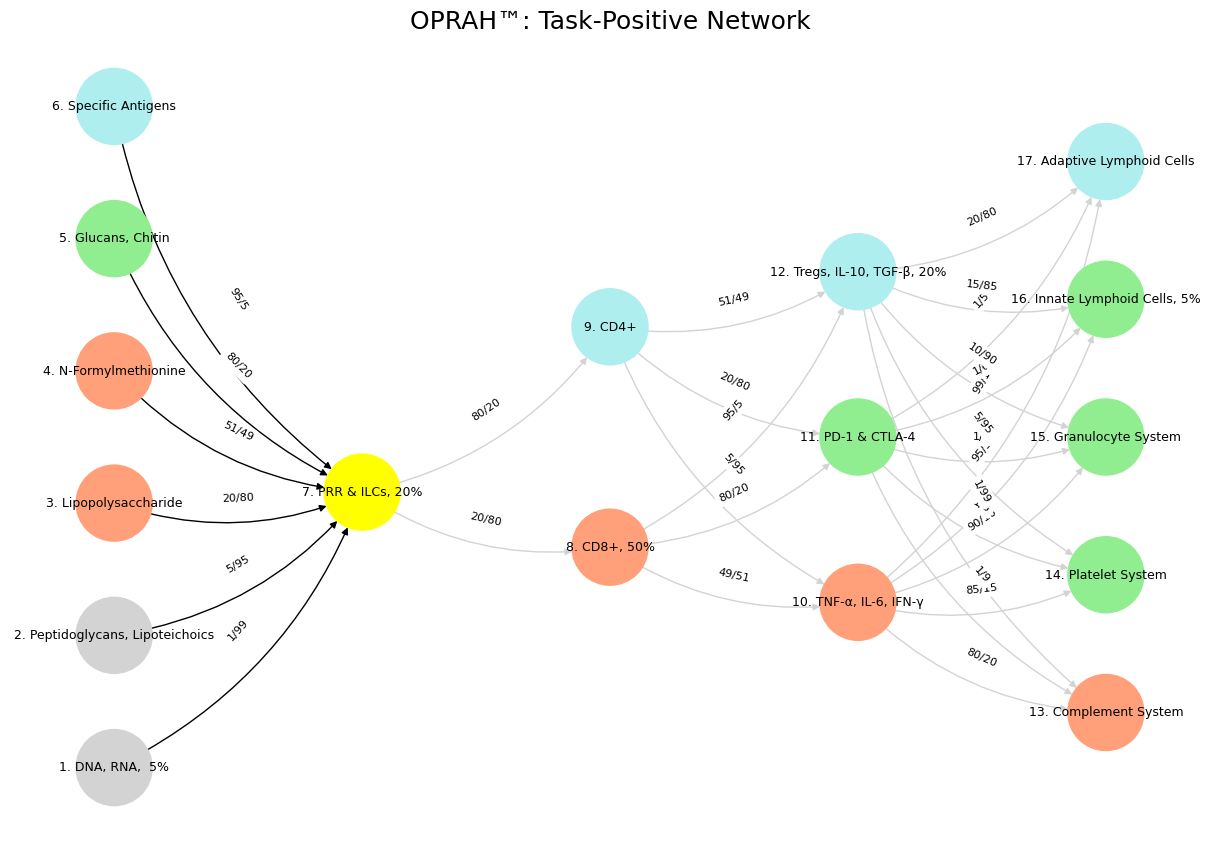
Fig. 39 Space is Apollonian and Time Dionysian. They are the static representation and the dynamic emergent. Ain’t that somethin?