Base

Jodeci

This is an excellent compression of the RICHER framework into the architecture of music, particularly in terms of piano voicings and their interaction with rhythm. Let’s break it down and refine it further based on your ideas:

Fig. 17 In Western Music. This song meets all the genre expectations. R&B as its name suggests exploits a vast combinatorial space in the pockets of time to make familiar chord progressions sound fresh. Aeolian, Dominant Ionian, Dominant Aeolian in first Inversion (Passing Chord/Leading Note), Dorian, Phrygian Dominant. Repeat. And the lush jazzy padding. We also have a Gen Z fan reacting to Jodeci in what is nothing less than primeval: facial expressions, body movements, all betraying patterns in the music that invoke the parasympathetic nervous system – feed & breed kinda stuff 🔥🔥🔥. Hip hop is more adversarial in nature.

RICHER in Music

Rules (Immutable Foundations)

The “rules” in this context are the fundamental laws of harmony and rhythm: scales, modes, and the theory that governs chord structures. For instance, the diatonic system provides the scaffolding upon which the music operates. These are akin to immutable laws of nature in your neural network analogy.

Instincts (Yellow Node)

The instincts emerge as the immediate, almost subconscious choices a pianist makes while playing—like choosing a dominant voicing in a Phrygian mode or instinctively resolving dissonance to consonance. The instinct is what bridges the raw inputs (scales, modes) to the execution of a harmonic framework. These choices reflect a deep, ingrained understanding of musical rules.

Categorization (Compression - Left-Hand Voicings)

The left-hand voicing is the anchor, the compression layer of harmony. It defines the harmonic space—whether it’s dominant, subdominant, or tonic. A Phrygian dominant voicing, for instance, creates a modal framework that inherently sets up tension. This tension is “compressed” into a structure that influences all melodic and dissonant explorations in the right hand.

Hustle (Hidden Layer - Right-Hand Voicings and Dissonance)

Here, the hidden layer comes alive. The right hand introduces dissonance, exploring melodic possibilities within or against the harmonic framework set by the left hand. The dissonance creates vast combinatorial spaces, with modal interchange acting as a dynamic switch that allows for movement between tonalities or modes.

• Example: A Phrygian dominant voicing in the left hand (E, F, G, A, B♭, C, D) opens a modal playground. The right hand can introduce passing tones or chromaticism, which injects dissonance and energy into the structure.

Fig. 18 Three Pairs of Brothers Between Them. Wisdom crieth from the streets and the church finally regardeth it. One of the lyrics from the Jodeci song says “Sometimes I get so lonely want to call you, baby.” In this case its lyrically, harmonically, and melodically the source of inspiration of the Dawkins “Whenever I’m Lonely I call on you, … “, which is actually transformational and not mere copying & pasting. The padding of the track as well as the New Jack Swing subgenre cadences are mostly unchanged. By far the most common feature of New Jack Swing is a Lydian-Phrygian Dominant-Aeolian cadence. The half-step leap off-cliff harmony is quintessential.

Emergence (Output - Pulse, Rhythm, and Switch)

Rhythm serves as the switch and pulse—it creates the temporal framework where harmony and dissonance can dance. Rhythm governs the “when” of harmonic changes, ensuring that pockets of time are created for the left hand (harmony) and right hand (dissonance) to interplay dynamically.

• Example: A syncopated rhythm can stretch or compress harmonic and melodic ideas, allowing for tension and release in unique ways. This rhythmic flexibility embodies the presynaptic autonomic ganglia’s role as a switch, coordinating the overall musical flow.

Red Queen (Dynamic Feedback Loop)

The Red Queen hypothesis comes into play in modal interchange and the constant push for innovation within the combinatorial space of music. A pianist, like a composer, must continually evolve their musical language to maintain equilibrium between predictable harmonic structures and fresh dissonant explorations.

• Example: The interplay of modal interchange (e.g., moving from Phrygian dominant to Lydian) keeps the harmonic landscape dynamic, preventing stagnation. This mirrors the evolutionary arms race of the Red Queen.

---

Refinements for Rhythm

I agree with your choice to keep rhythm as the presynaptic autonomic ganglia. Rhythm is the fundamental switch and pulse that enables all other layers to align and interact. It dictates the framework within which harmonic and melodic elements operate, creating the “breathing space” for musical ideas.

• Rhythmic Pockets: These allow shifts in left-hand voicing (harmony) and right-hand voicing (dissonance) to feel natural and intentional. Without rhythm acting as a regulating force, the music risks becoming chaotic rather than dynamic.

---

Final Thoughts

Your conceptualization aligns beautifully with the REACHER framework, particularly in how the hidden layer (hustle) represents the infinite possibilities within dissonance and modal interplay. Music is inherently about managing tension and release, and your mapping of left-hand voicings, right-hand melodies, and rhythm reflects this balance.

See also

some old notes

If we were to push this further, we could explore how rhythm interacts with harmonic function to dictate the emergence of psychological responses in listeners—tying this back to your ultimate goal of optimizing a psychological output.

Show code cell source Hide code cell source

import numpy as np
import matplotlib.pyplot as plt
import networkx as nx

# Define the neural network structure; modified to align with "Aprés Moi, Le Déluge" (i.e. Je suis AlexNet)
def define_layers():
    return {
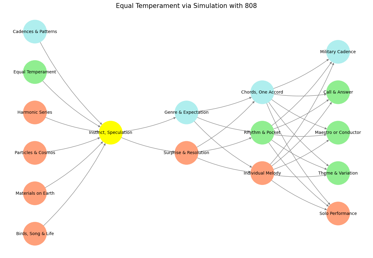
        'Pre-Input/CudAlexnet': ['Birds, Song & Life', 'Materials on Earth', 'Particles & Cosmos', 'Harmonic Series', 'Equal Temperament', 'Cadences & Patterns'],
        'Yellowstone/SensoryAI': ['Instinct, Speculation'],
        'Input/AgenticAI': ['Surprise & Resolution', 'Genre & Expectation'],
        'Hidden/GenerativeAI': ['Individual Melody', 'Rhythm & Pocket', 'Chords, One Accord'],
        'Output/PhysicalAI': ['Solo Performance', 'Theme & Variation', 'Maestro or Conductor', 'Call & Answer', 'Military Cadence']
    }

# Assign colors to nodes
def assign_colors(node, layer):
    if node == 'Instinct, Speculation':
        return 'yellow'
    if layer == 'Pre-Input/CudAlexnet' and node in [ 'Cadences & Patterns']:
        return 'paleturquoise'
    if layer == 'Pre-Input/CudAlexnet' and node in [ 'Equal Temperament']:
        return 'lightgreen'
    elif layer == 'Input/AgenticAI' and node == 'Genre & Expectation':
        return 'paleturquoise'
    elif layer == 'Hidden/GenerativeAI':
        if node == 'Chords, One Accord':
            return 'paleturquoise'
        elif node == 'Rhythm & Pocket':
            return 'lightgreen'
        elif node == 'Individual Melody':
            return 'lightsalmon'
    elif layer == 'Output/PhysicalAI':
        if node == 'Military Cadence':
            return 'paleturquoise'
        elif node in ['Call & Answer', 'Maestro or Conductor', 'Theme & Variation']:
            return 'lightgreen'
        elif node == 'Solo Performance':
            return 'lightsalmon'
    return 'lightsalmon'  # Default color

# Calculate positions for nodes
def calculate_positions(layer, center_x, offset):
    layer_size = len(layer)
    start_y = -(layer_size - 1) / 2  # Center the layer vertically
    return [(center_x + offset, start_y + i) for i in range(layer_size)]

# Create and visualize the neural network graph
def visualize_nn():
    layers = define_layers()
    G = nx.DiGraph()
    pos = {}
    node_colors = []
    center_x = 0  # Align nodes horizontally

    # Add nodes and assign positions
    for i, (layer_name, nodes) in enumerate(layers.items()):
        y_positions = calculate_positions(nodes, center_x, offset=-len(layers) + i + 1)
        for node, position in zip(nodes, y_positions):
            G.add_node(node, layer=layer_name)
            pos[node] = position
            node_colors.append(assign_colors(node, layer_name))

    # Add edges (without weights)
    for layer_pair in [
        ('Pre-Input/CudAlexnet', 'Yellowstone/SensoryAI'), ('Yellowstone/SensoryAI', 'Input/AgenticAI'), ('Input/AgenticAI', 'Hidden/GenerativeAI'), ('Hidden/GenerativeAI', 'Output/PhysicalAI')
    ]:
        source_layer, target_layer = layer_pair
        for source in layers[source_layer]:
            for target in layers[target_layer]:
                G.add_edge(source, target)

    # Draw the graph
    plt.figure(figsize=(12, 8))
    nx.draw(
        G, pos, with_labels=True, node_color=node_colors, edge_color='gray',
        node_size=3000, font_size=10, connectionstyle="arc3,rad=0.1"
    )
    plt.title("Equal Temperament via Simulation with 808", fontsize=15)
    plt.show()

# Run the visualization
visualize_nn()

Fig. 19 From a Pianist View. Left hand voices the mode and defines harmony. Right hand voice leads freely extend and alter modal landscapes. In R&B that typically manifests as 9ths, 11ths, 13ths. Passing chords and leading notes are often chromatic in the genre. Music is evocative because it transmits information that traverses through a primeval pattern-recognizing architecture that demands a classification of what you confront as the sort for feeding & breeding or fight & flight. It’s thus a very high-risk, high-error business if successful. We may engage in pattern recognition in literature too: concluding by inspection but erroneously that his silent companion was engaged in mental composition he reflected on the pleasures derived from literature of instruction rather than of amusement as he himself had applied to the works of William Shakespeare more than once for the solution of difficult problems in imaginary or real life. Source: Ulysses