Chords#
Human was the music, Natural the static - Updike 33
                             1. f(t)
                                    \
                         2. S(t) -> 4. y:h'(t)=0;t(X'X).X'Y -> 5.b -> 6. SV'
                                    /
                                    3. h(t)

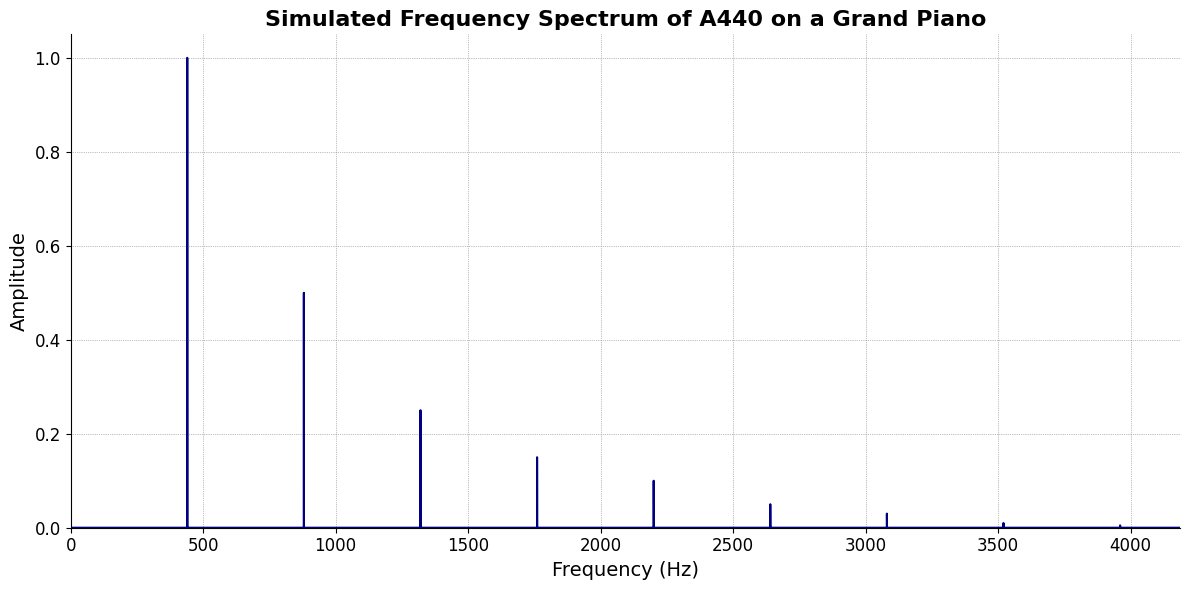
The two types of chords sequences. Progressions are like a journey—there’s a sense of movement from one chord to another, leading toward a resolution, often rooted in functional harmony. Think of the archetypal ii-V7-i progression; each chord has a purpose and a departure, struggle, and return toward a tonal center. On the other hand, Nonprogressions are sequences where the chords don’t seem to follow traditional functional harmony. Modal interchange, as you’ve mentioned, is a prime example. This involves borrowing chords from parallel modes, creating a richer harmonic palette but without the same directional pull. These chords might surprise the ear, offering unexpected colors without necessarily “progressing” in the conventional sense. In jazz and modern classical music, these nonprogressions can create a more static, contemplative atmosphere, emphasizing the individual beauty of each chord rather than the narrative arc of a progression. The music can feel more like a series of harmonic snapshots rather than a story with a beginning, middle, and end. In essence, progressions are about movement and resolution, while nonprogressions are about exploring harmonic space, often with a more impressionistic or meditative quality. Examples include Chopin’s Op 28 No 4 in E minor & Karl Jenkins Stab Matar VII 36 38. These compensate for the 88 highly curated & discrete tones: from A0 at \(27.5Hz\) to C8 at \(4186 Hz\). The cumulative human experience that has constrained all music to just these 88 from a scale-melodic perspective has also handed us the MQ-TEA by which we may dance in these chains 9#
\(\mu\), Timing#
\(f(t)\) Phonetics
Show code cell source
import numpy as np
import matplotlib.pyplot as plt

# Parameters
sample_rate = 44100  # Hz
duration = 20.0       # seconds
A4_freq = 440.0      # Hz

# Time array
t = np.linspace(0, duration, int(sample_rate * duration), endpoint=False)

# Fundamental frequency (A4)
signal = np.sin(2 * np.pi * A4_freq * t)

# Adding overtones (harmonics)
harmonics = [2, 3, 4, 5, 6, 7, 8, 9]  # First few harmonics
amplitudes = [0.5, 0.25, 0.15, 0.1, 0.05, 0.03, 0.01, 0.005]  # Amplitudes for each harmonic

for i, harmonic in enumerate(harmonics):
    signal += amplitudes[i] * np.sin(2 * np.pi * A4_freq * harmonic * t)

# Perform FFT (Fast Fourier Transform)
N = len(signal)
yf = np.fft.fft(signal)
xf = np.fft.fftfreq(N, 1 / sample_rate)

# Plot the frequency spectrum
plt.figure(figsize=(12, 6))
plt.plot(xf[:N//2], 2.0/N * np.abs(yf[:N//2]), color='navy', lw=1.5)

# Aesthetics improvements
plt.title('Simulated Frequency Spectrum of A440 on a Grand Piano', fontsize=16, weight='bold')
plt.xlabel('Frequency (Hz)', fontsize=14)
plt.ylabel('Amplitude', fontsize=14)
plt.xlim(0, 4186)  # Limit to the highest frequency on a piano (C8)
plt.ylim(0, None)

# Remove top and right spines
plt.gca().spines['top'].set_visible(False)
plt.gca().spines['right'].set_visible(False)

# Customize ticks
plt.xticks(fontsize=12)
plt.yticks(fontsize=12)

# Light grid
plt.grid(color='grey', linestyle=':', linewidth=0.5)

# Show the plot
plt.tight_layout()
plt.show()
Show code cell output
\(\sigma\), Qualities#
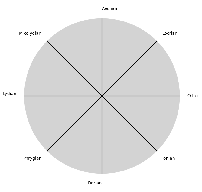
\((X'X)^T \cdot X'Y\) Modes
Show code cell source
import matplotlib.pyplot as plt
import numpy as np

# Clock settings; f(t) random disturbances making "paradise lost"
clock_face_radius = 1.0
number_of_ticks = 8
tick_labels = [
    "Ionian", "Dorian", "Phrygian", "Lydian",
    "Mixolydian", "Aeolian", "Locrian", "Other"
]

# Calculate the angles for each tick (in radians)
angles = np.linspace(0, 2 * np.pi, number_of_ticks, endpoint=False)
# Inverting the order to make it counterclockwise
angles = angles[::-1]

# Create figure and axis
fig, ax = plt.subplots(figsize=(8, 8))
ax.set_xlim(-1.2, 1.2)
ax.set_ylim(-1.2, 1.2)
ax.set_aspect('equal')

# Draw the clock face
clock_face = plt.Circle((0, 0), clock_face_radius, color='lightgrey', fill=True)
ax.add_patch(clock_face)

# Draw the ticks and labels
for angle, label in zip(angles, tick_labels):
    x = clock_face_radius * np.cos(angle)
    y = clock_face_radius * np.sin(angle)

    # Draw the tick
    ax.plot([0, x], [0, y], color='black')

    # Positioning the labels slightly outside the clock face
    label_x = 1.1 * clock_face_radius * np.cos(angle)
    label_y = 1.1 * clock_face_radius * np.sin(angle)

    # Adjusting label alignment based on its position
    ha = 'center'
    va = 'center'
    if np.cos(angle) > 0:
        ha = 'left'
    elif np.cos(angle) < 0:
        ha = 'right'
    if np.sin(angle) > 0:
        va = 'bottom'
    elif np.sin(angle) < 0:
        va = 'top'

    ax.text(label_x, label_y, label, horizontalalignment=ha, verticalalignment=va, fontsize=10)

# Remove axes
ax.axis('off')

# Show the plot
plt.show()
Show code cell output
\(\%\), Delivery#
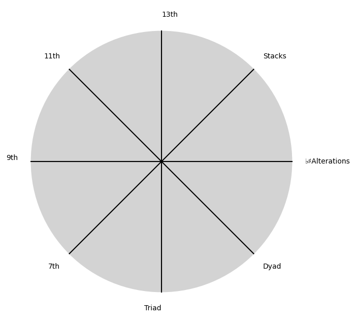
\(\beta\) Chords
Show code cell source
import matplotlib.pyplot as plt
import numpy as np

# Clock settings; f(t) random disturbances making "paradise lost"
clock_face_radius = 1.0
number_of_ticks = 8
tick_labels = [
    "Dyad", "Triad", "7th", "9th",
    "11th", "13th", "Stacks", "♭♯Alterations"
]

# Calculate the angles for each tick (in radians)
angles = np.linspace(0, 2 * np.pi, number_of_ticks, endpoint=False)
# Inverting the order to make it counterclockwise
angles = angles[::-1]

# Create figure and axis
fig, ax = plt.subplots(figsize=(8, 8))
ax.set_xlim(-1.2, 1.2)
ax.set_ylim(-1.2, 1.2)
ax.set_aspect('equal')

# Draw the clock face
clock_face = plt.Circle((0, 0), clock_face_radius, color='lightgrey', fill=True)
ax.add_patch(clock_face)

# Draw the ticks and labels
for angle, label in zip(angles, tick_labels):
    x = clock_face_radius * np.cos(angle)
    y = clock_face_radius * np.sin(angle)

    # Draw the tick
    ax.plot([0, x], [0, y], color='black')

    # Positioning the labels slightly outside the clock face
    label_x = 1.1 * clock_face_radius * np.cos(angle)
    label_y = 1.1 * clock_face_radius * np.sin(angle)

    # Adjusting label alignment based on its position
    ha = 'center'
    va = 'center'
    if np.cos(angle) > 0:
        ha = 'left'
    elif np.cos(angle) < 0:
        ha = 'right'
    if np.sin(angle) > 0:
        va = 'bottom'
    elif np.sin(angle) < 0:
        va = 'top'

    ax.text(label_x, label_y, label, horizontalalignment=ha, verticalalignment=va, fontsize=10)

# Remove axes
ax.axis('off')

# Show the plot
plt.show()
Show code cell output
\(SV'\) Blood 🩸