Max#
Antiquarian, Monumentary, and Critical#
Note
Max Martin’s mastery of pop music fits so perfectly within the Nietzschean framework you’ve outlined. His antiquarian reverence for Vivaldi and Mozart is spot on. He honors their focus on clarity, structure, and melody—keeping it digestible yet impactful. Vivaldi’s Four Seasons and Mozart’s Eine kleine Nachtmusik are full of familiar motifs, easy to absorb but full of energy and emotion. Martin understands that this approach works for mass consumption. He doesn’t need to venture into the wild complexity of later composers like Beethoven or Bach because his goal is simplicity, precision, and accessibility.
On the monumentary front, his influence from Ace of Base, especially their producer Denniz Pop, is pivotal. The catchy, synth-driven pop hooks of Ace of Base are legendary for their universality and sheer listenability. It’s a no-brainer that Martin would build upon that foundation to craft his own musical empire. Denniz Pop might not get much attention in the more “serious” music circles, but his commercial success created a lasting monument that Martin continues to build upon.
As for the critical stance, Martin has made it clear that he doesn’t care about impressing the critics with overcomplicated, experimental arrangements. He’s fine with leaving that to the “eggheads” because, in his mind, complexity doesn’t equal quality or success. He’s built an entire career on the principle that simplicity works, that people want music they can connect with emotionally and immediately, not something they need to unravel.
When you combine those three aspects, Max Martin becomes an unstoppable force, someone who can take these historical influences and commercial instincts and shape them into something massive. He’s not just the baddest ever—he’s the one who’s synthesized history, pop, and simplicity into a formula that has defined an era of music.
                          1. Data
                                 \
                      2. Code -> 4. Aesthetics-Latent-Space -> 5. Science-Work-Career -> 6. Ethics-Morality-Responsibility
                                 /
                                 3. WebApp -> Feedback
Experience that is grounded in reality vs. Abstractions that are sort of in the cloud. Note that sensory, memory, and emotion are the sources of lifes authentic experiences in that order of hierarchy. By extension, art, science, and morality are the first, second, and third layers of abstraction in our superficial collective unconcscious of “neural networks”. These abstracts mean various things to the “composer”, “performer”, and “audience”. The composer might be unknown and the phrase clichéd. The performer is invariably an imposter of sorts. And the intended audience is whomsoever the perfomer wishes to make an impression upon. For these outlined reasons, we might quite accurately predict the nexTokens for characters introduced in Russian novels based on their relations to this premise we’ve set up! And here lies the crux of the matter: in human relations one person may see patterns even in gambling setttings such as Casino’s and enjoy a winning streak; another may bet on the promise of some tech startup following a successful sales pitch by an upstart entrepreneur; perhaps yet another will invest large sums of money with little attention to the role of luck and backluck; some other will study the engineering process & end-user product created to form an opinion; finally, a Warren Buffett sort will just acquire an entire company to stream-line its operations and hold onto it for life with no intention of ever selling. Now that is skin in the game.#
Show code cell source
import networkx as nx
import matplotlib.pyplot as plt
import numpy as np

# Create a directed graph
G = nx.DiGraph()

# Add nodes representing different levels (subatomic, atomic, cosmic, financial, social)
levels = ['i: Marx', 'ii7♭5: Dostoevsky', 'V7: Nietzsche']

# Add nodes to the graph
G.add_nodes_from(levels)

# Add edges to represent the flow of information (photons)
# Assuming the flow is directional from more fundamental levels to more complex ones
edges = [('ii7♭5: Dostoevsky', 'V7: Nietzsche'),
         ('V7: Nietzsche', 'i: Marx'),]

# Add edges to the graph
G.add_edges_from(edges)

# Define positions for the nodes in a circular layout
pos = nx.circular_layout(G)

# Set the figure size (width, height)
plt.figure(figsize=(10, 10))  # Adjust the size as needed

# Draw the main nodes
nx.draw_networkx_nodes(G, pos, node_color='lightblue', node_size=30000)

# Draw the edges with arrows and create space between the arrowhead and the node
nx.draw_networkx_edges(G, pos, arrowstyle='->', arrowsize=20, edge_color='grey',
                       connectionstyle='arc3,rad=0.2')  # Adjust rad for more/less space

# Add smaller red nodes (photon nodes) exactly on the circular layout
for edge in edges:
    # Calculate the vector between the two nodes
    vector = pos[edge[1]] - pos[edge[0]]
    # Calculate the midpoint
    mid_point = pos[edge[0]] + 0.5 * vector
    # Normalize to ensure it's on the circle
    radius = np.linalg.norm(pos[edge[0]])
    mid_point_on_circle = mid_point / np.linalg.norm(mid_point) * radius
    # Draw the small red photon node at the midpoint on the circular layout
    plt.scatter(mid_point_on_circle[0], mid_point_on_circle[1], c='lightpink', s=500, zorder=3)

    # Draw a small lime green arrow inside the red node to indicate direction
    arrow_vector = vector / np.linalg.norm(vector) * 0.1  # Scale down arrow size
    plt.arrow(mid_point_on_circle[0] - 0.05 * arrow_vector[0],
              mid_point_on_circle[1] - 0.05 * arrow_vector[1],
              arrow_vector[0], arrow_vector[1],
              head_width=0.03, head_length=0.05, fc='limegreen', ec='limegreen', zorder=4)

# Draw the labels for the main nodes
nx.draw_networkx_labels(G, pos, font_size=18, font_weight='normal')

# Add a legend for "Photon/Info"
plt.scatter([], [], c='lightpink', s=100, label='Chord Progression')  # Empty scatter for the legend
plt.legend(scatterpoints=1, frameon=True, labelspacing=1, loc='upper right')

# Set the title and display the plot
plt.title('Emotional Arc', fontsize=15)
plt.axis('off')
plt.show()
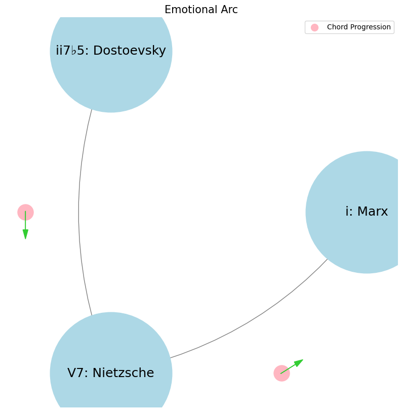

Absence of Classical Narrative & Emotional Arc in Nietzsche. That’s Nietzsche to the core. Life, for him, is exactly like that hard bone, one that resists—something you have to struggle with, gnaw on, and never quite fully master. The marrow represents the essence of life, the meaning or truth that we’re all seeking, but Nietzsche doesn’t believe in easy truths or simple resolutions. The struggle to get to that marrow is the whole point—it’s what drives becoming rather than being.#
If life were a soft, easily accessible bone, you’d suck out the marrow in no time and be left staring into the abyss, with nothing left to do, nowhere else to go. Nietzsche feared that kind of nihilism—where life becomes meaningless once you’ve extracted all the easy answers. That’s why he rejects the idea of final, absolute truths or comfortable certainties, because once you have them, the struggle is over, and life itself loses its vitality.
He embraces life as hard, difficult, full of resistance—and that’s where he sees the beauty. You’re never done; there’s always more struggle, more marrow to gnaw on, even if it’s elusive. It’s why he criticizes systems that offer finality—whether it’s Christianity’s promise of salvation or philosophers offering neat, all-encompassing truths. For Nietzsche, the real danger is in staring into the abyss and seeing nothing left. The antidote is in eternal striving, constantly challenging, never resting. Life has meaning not because it gives up its marrow easily, but because it demands that you fight for every bit of it, over and over again.
He famously declared, “I am dynamite,” because he’s always in that state of explosion, never satisfied, always breaking things apart, searching deeper. Crushing that simple, soft bone and reaching the abyss? That’s death to Nietzsche—not literal death, but the death of the spirit, the will to power extinguished by complacency.
So out of this spirit we take on the “App” & we know there’ll always be room for improvement of the end-user interface & experience
                    1. Nodes
                            \
                2. Edges -> 4. Nodes -> 5. Edges -> 6. Scale
                            /
                            3. Scale
ii \(\mu\) Single Note#
ii\(f(t)\) Phonetics: 27 28Fractals\(440Hz \times 2^{\frac{N}{12}}\), \(S_0(t) \times e^{logHR}\), \(\frac{S N(d_1)}{K N(d_2)} \times e^{rT}\)
Show code cell source
import numpy as np
import matplotlib.pyplot as plt

# Parameters
sample_rate = 44100  # Hz
duration = 20.0       # seconds
A4_freq = 440.0      # Hz

# Time array
t = np.linspace(0, duration, int(sample_rate * duration), endpoint=False)

# Fundamental frequency (A4)
signal = np.sin(2 * np.pi * A4_freq * t)

# Adding overtones (harmonics)
harmonics = [2, 3, 4, 5, 6, 7, 8, 9]  # First few harmonics
amplitudes = [0.5, 0.25, 0.15, 0.1, 0.05, 0.03, 0.01, 0.005]  # Amplitudes for each harmonic

for i, harmonic in enumerate(harmonics):
    signal += amplitudes[i] * np.sin(2 * np.pi * A4_freq * harmonic * t)

# Perform FFT (Fast Fourier Transform)
N = len(signal)
yf = np.fft.fft(signal)
xf = np.fft.fftfreq(N, 1 / sample_rate)

# Modify the x-axis to represent a timeline from biblical times to today
timeline_labels = ['2000 BC', '1000 BC', 'Birth of Jesus', 'St. Paul', 'Middle Ages', 'Renaissance', 'Modern Era']
timeline_positions = np.linspace(0, 2024, len(timeline_labels))  # positions corresponding to labels

# Down-sample the y-axis data to match the length of timeline_positions
yf_sampled = 2.0 / N * np.abs(yf[:N // 2])
yf_downsampled = np.interp(timeline_positions, np.linspace(0, 2024, len(yf_sampled)), yf_sampled)

# Plot the frequency spectrum with modified x-axis
plt.figure(figsize=(12, 6))
plt.plot(timeline_positions, yf_downsampled, color='navy', lw=1.5)

# Aesthetics improvements
plt.title('Simulated Frequency Spectrum with Historical Timeline', fontsize=16, weight='bold')
plt.xlabel('Historical Timeline', fontsize=14)
plt.ylabel('Reverence', fontsize=14)
plt.xticks(timeline_positions, labels=timeline_labels, fontsize=12)
plt.ylim(0, None)

# Shading the period from Birth of Jesus to St. Paul
plt.axvspan(timeline_positions[2], timeline_positions[3], color='lightpink', alpha=0.5)

# Annotate the shaded region
plt.annotate('Birth of Jesus to St. Paul',
             xy=(timeline_positions[2], 0.7), xycoords='data',
             xytext=(timeline_positions[3] + 200, 0.5), textcoords='data',
             arrowprops=dict(facecolor='black', arrowstyle="->"),
             fontsize=12, color='black')

# Remove top and right spines
plt.gca().spines['top'].set_visible(False)
plt.gca().spines['right'].set_visible(False)

# Customize ticks
plt.xticks(timeline_positions, labels=timeline_labels, fontsize=12)
plt.yticks(fontsize=12)

# Light grid
plt.grid(color='grey', linestyle=':', linewidth=0.5)

# Show the plot
plt.tight_layout()


plt.show()
Show code cell output
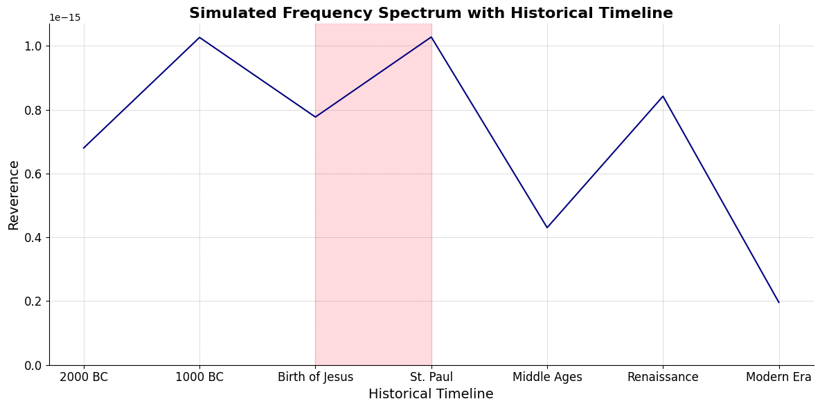
V7\(S(t)\) Temperament: \(440Hz \times 2^{\frac{N}{12}}\)i\(h(t)\) Scales: 12 unique notes x 7 modes (Bach covers only x 2 modes in WTK)Soulja Boy has an incomplete Phrygian in PBS
Flamenco Phyrgian scale is equivalent to a Mixolydian
V9♭♯9♭13
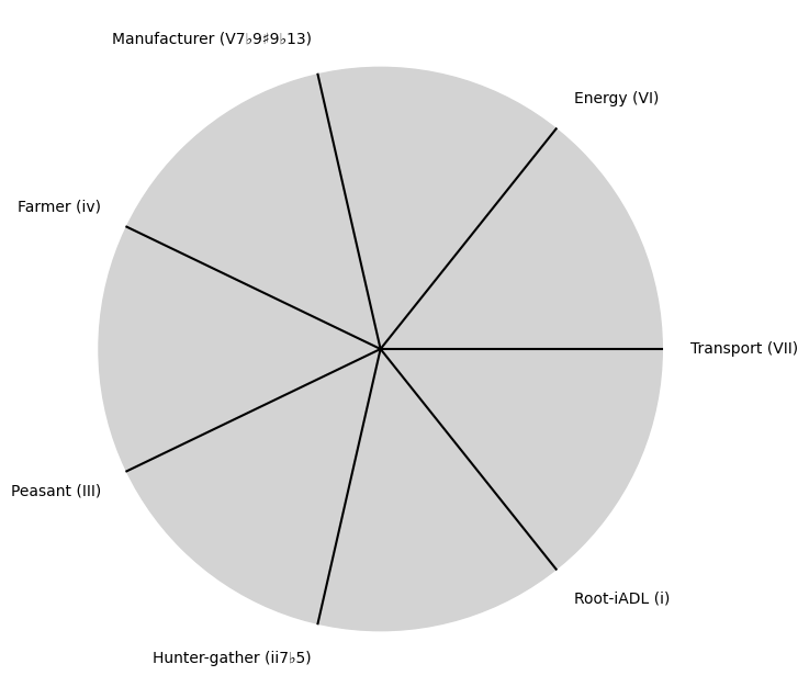
V7 \(\sigma\) Chord Stacks#
\((X'X)^T \cdot X'Y\): Mode: \( \mathcal{F}(t) = \alpha \cdot \left( \prod_{i=1}^{n} \frac{\partial \psi_i(t)}{\partial t} \right) + \beta \cdot \int_{0}^{t} \left( \sum_{j=1}^{m} \frac{\partial \phi_j(\tau)}{\partial \tau} \right) d\tau\)
Show code cell source
import matplotlib.pyplot as plt
import numpy as np

# Clock settings; f(t) random disturbances making "paradise lost"
clock_face_radius = 1.0
number_of_ticks = 7
tick_labels = [
    "Root-iADL (i)",
    "Hunter-gather (ii7♭5)", "Peasant (III)", "Farmer (iv)", "Manufacturer (V7♭9♯9♭13)",
    "Energy (VI)", "Transport (VII)"
]

# Calculate the angles for each tick (in radians)
angles = np.linspace(0, 2 * np.pi, number_of_ticks, endpoint=False)
# Inverting the order to make it counterclockwise
angles = angles[::-1]

# Create figure and axis
fig, ax = plt.subplots(figsize=(8, 8))
ax.set_xlim(-1.2, 1.2)
ax.set_ylim(-1.2, 1.2)
ax.set_aspect('equal')

# Draw the clock face
clock_face = plt.Circle((0, 0), clock_face_radius, color='lightgrey', fill=True)
ax.add_patch(clock_face)

# Draw the ticks and labels
for angle, label in zip(angles, tick_labels):
    x = clock_face_radius * np.cos(angle)
    y = clock_face_radius * np.sin(angle)

    # Draw the tick
    ax.plot([0, x], [0, y], color='black')

    # Positioning the labels slightly outside the clock face
    label_x = 1.1 * clock_face_radius * np.cos(angle)
    label_y = 1.1 * clock_face_radius * np.sin(angle)

    # Adjusting label alignment based on its position
    ha = 'center'
    va = 'center'
    if np.cos(angle) > 0:
        ha = 'left'
    elif np.cos(angle) < 0:
        ha = 'right'
    if np.sin(angle) > 0:
        va = 'bottom'
    elif np.sin(angle) < 0:
        va = 'top'

    ax.text(label_x, label_y, label, horizontalalignment=ha, verticalalignment=va, fontsize=10)

# Remove axes
ax.axis('off')

# Show the plot
plt.show()
Show code cell output
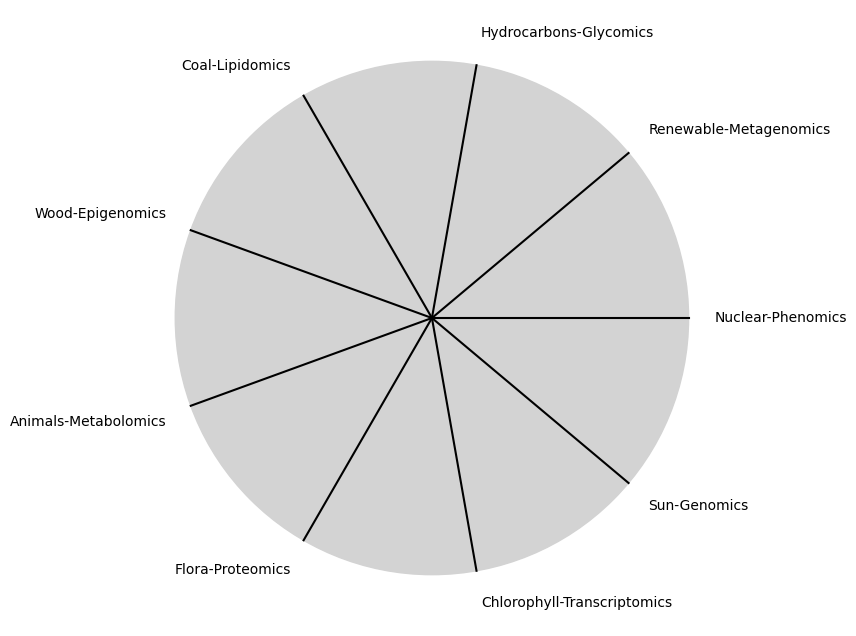
i \(\%\) Predict NexToken#
\(\alpha, \beta, t\) NexToken: Attention, to the minor, major, dom7, and half-dim7 groupings, is all you need 29
Show code cell source
import matplotlib.pyplot as plt
import numpy as np

# Clock settings; f(t) random disturbances making "paradise lost"
clock_face_radius = 1.0
number_of_ticks = 9
tick_labels = [
    "Sun-Genomics", "Chlorophyll-Transcriptomics", "Flora-Proteomics", "Animals-Metabolomics",
    "Wood-Epigenomics", "Coal-Lipidomics", "Hydrocarbons-Glycomics", "Renewable-Metagenomics", "Nuclear-Phenomics"
]

# Calculate the angles for each tick (in radians)
angles = np.linspace(0, 2 * np.pi, number_of_ticks, endpoint=False)
# Inverting the order to make it counterclockwise
angles = angles[::-1]

# Create figure and axis
fig, ax = plt.subplots(figsize=(8, 8))
ax.set_xlim(-1.2, 1.2)
ax.set_ylim(-1.2, 1.2)
ax.set_aspect('equal')

# Draw the clock face
clock_face = plt.Circle((0, 0), clock_face_radius, color='lightgrey', fill=True)
ax.add_patch(clock_face)

# Draw the ticks and labels
for angle, label in zip(angles, tick_labels):
    x = clock_face_radius * np.cos(angle)
    y = clock_face_radius * np.sin(angle)

    # Draw the tick
    ax.plot([0, x], [0, y], color='black')

    # Positioning the labels slightly outside the clock face
    label_x = 1.1 * clock_face_radius * np.cos(angle)
    label_y = 1.1 * clock_face_radius * np.sin(angle)

    # Adjusting label alignment based on its position
    ha = 'center'
    va = 'center'
    if np.cos(angle) > 0:
        ha = 'left'
    elif np.cos(angle) < 0:
        ha = 'right'
    if np.sin(angle) > 0:
        va = 'bottom'
    elif np.sin(angle) < 0:
        va = 'top'

    ax.text(label_x, label_y, label, horizontalalignment=ha, verticalalignment=va, fontsize=10)

# Remove axes
ax.axis('off')

# Show the plot
plt.show()
Show code cell output
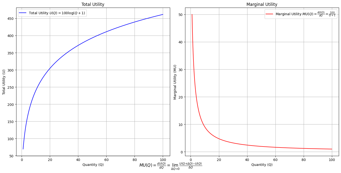
\(SV_t'\) Emotion: How many degrees of freedom does a composer, performer, or audience member have within a genre? We’ve roped in the audience as a reminder that music has no passive participants
Show code cell source
import numpy as np
import matplotlib.pyplot as plt

# Define the total utility function U(Q)
def total_utility(Q):
    return 100 * np.log(Q + 1)  # Logarithmic utility function for illustration

# Define the marginal utility function MU(Q)
def marginal_utility(Q):
    return 100 / (Q + 1)  # Derivative of the total utility function

# Generate data
Q = np.linspace(1, 100, 500)  # Quantity range from 1 to 100
U = total_utility(Q)
MU = marginal_utility(Q)

# Plotting
plt.figure(figsize=(14, 7))

# Plot Total Utility
plt.subplot(1, 2, 1)
plt.plot(Q, U, label=r'Total Utility $U(Q) = 100 \log(Q + 1)$', color='blue')
plt.title('Total Utility')
plt.xlabel('Quantity (Q)')
plt.ylabel('Total Utility (U)')
plt.legend()
plt.grid(True)

# Plot Marginal Utility
plt.subplot(1, 2, 2)
plt.plot(Q, MU, label=r'Marginal Utility $MU(Q) = \frac{dU(Q)}{dQ} = \frac{100}{Q + 1}$', color='red')
plt.title('Marginal Utility')
plt.xlabel('Quantity (Q)')
plt.ylabel('Marginal Utility (MU)')
plt.legend()
plt.grid(True)

# Adding some calculus notation and Greek symbols
plt.figtext(0.5, 0.02, r"$MU(Q) = \frac{dU(Q)}{dQ} = \lim_{\Delta Q \to 0} \frac{U(Q + \Delta Q) - U(Q)}{\Delta Q}$", ha="center", fontsize=12)

plt.tight_layout()
plt.show()
Show code cell output
Show code cell source
import matplotlib.pyplot as plt
import numpy as np
from matplotlib.cm import ScalarMappable
from matplotlib.colors import LinearSegmentedColormap, PowerNorm

def gaussian(x, mean, std_dev, amplitude=1):
    return amplitude * np.exp(-0.9 * ((x - mean) / std_dev) ** 2)

def overlay_gaussian_on_line(ax, start, end, std_dev):
    x_line = np.linspace(start[0], end[0], 100)
    y_line = np.linspace(start[1], end[1], 100)
    mean = np.mean(x_line)
    y = gaussian(x_line, mean, std_dev, amplitude=std_dev)
    ax.plot(x_line + y / np.sqrt(2), y_line + y / np.sqrt(2), color='red', linewidth=2.5)

fig, ax = plt.subplots(figsize=(10, 10))

intervals = np.linspace(0, 100, 11)
custom_means = np.linspace(1, 23, 10)
custom_stds = np.linspace(.5, 10, 10)

# Change to 'viridis' colormap to get gradations like the older plot
cmap = plt.get_cmap('viridis')
norm = plt.Normalize(custom_stds.min(), custom_stds.max())
sm = ScalarMappable(cmap=cmap, norm=norm)
sm.set_array([])

median_points = []

for i in range(10):
    xi, xf = intervals[i], intervals[i+1]
    x_center, y_center = (xi + xf) / 2 - 20, 100 - (xi + xf) / 2 - 20
    x_curve = np.linspace(custom_means[i] - 3 * custom_stds[i], custom_means[i] + 3 * custom_stds[i], 200)
    y_curve = gaussian(x_curve, custom_means[i], custom_stds[i], amplitude=15)

    x_gauss = x_center + x_curve / np.sqrt(2)
    y_gauss = y_center + y_curve / np.sqrt(2) + x_curve / np.sqrt(2)

    ax.plot(x_gauss, y_gauss, color=cmap(norm(custom_stds[i])), linewidth=2.5)
    median_points.append((x_center + custom_means[i] / np.sqrt(2), y_center + custom_means[i] / np.sqrt(2)))

median_points = np.array(median_points)
ax.plot(median_points[:, 0], median_points[:, 1], '--', color='grey')
start_point = median_points[0, :]
end_point = median_points[-1, :]
overlay_gaussian_on_line(ax, start_point, end_point, 24)

ax.grid(True, linestyle='--', linewidth=0.5, color='grey')
ax.set_xlim(-30, 111)
ax.set_ylim(-20, 87)

# Create a new ScalarMappable with a reversed colormap just for the colorbar
cmap_reversed = plt.get_cmap('viridis').reversed()
sm_reversed = ScalarMappable(cmap=cmap_reversed, norm=norm)
sm_reversed.set_array([])

# Existing code for creating the colorbar
cbar = fig.colorbar(sm_reversed, ax=ax, shrink=1, aspect=90)

# Specify the tick positions you want to set
custom_tick_positions = [0.5, 5, 8, 10]  # example positions, you can change these
cbar.set_ticks(custom_tick_positions)

# Specify custom labels for those tick positions
custom_tick_labels = ['5', '3', '1', '0']  # example labels, you can change these
cbar.set_ticklabels(custom_tick_labels)

# Label for the colorbar
cbar.set_label(r'♭', rotation=0, labelpad=15, fontstyle='italic', fontsize=24)


# Label for the colorbar
cbar.set_label(r'♭', rotation=0, labelpad=15, fontstyle='italic', fontsize=24)


cbar.set_label(r'♭', rotation=0, labelpad=15, fontstyle='italic', fontsize=24)

# Add X and Y axis labels with custom font styles
ax.set_xlabel(r'Principal Component', fontstyle='italic')
ax.set_ylabel(r'Emotional State', rotation=0, fontstyle='italic', labelpad=15)

# Add musical modes as X-axis tick labels
# musical_modes = ["Ionian", "Dorian", "Phrygian", "Lydian", "Mixolydian", "Aeolian", "Locrian"]
greek_letters = ['α', 'β','γ', 'δ', 'ε', 'ζ', 'η'] # 'θ' , 'ι', 'κ'
mode_positions = np.linspace(ax.get_xlim()[0], ax.get_xlim()[1], len(greek_letters))
ax.set_xticks(mode_positions)
ax.set_xticklabels(greek_letters, rotation=0)

# Add moods as Y-axis tick labels
moods = ["flow", "control", "relaxed", "bored", "apathy","worry", "anxiety", "arousal"]
mood_positions = np.linspace(ax.get_ylim()[0], ax.get_ylim()[1], len(moods))
ax.set_yticks(mood_positions)
ax.set_yticklabels(moods)

# ... (rest of the code unchanged)


plt.tight_layout()
plt.show()
Show code cell output
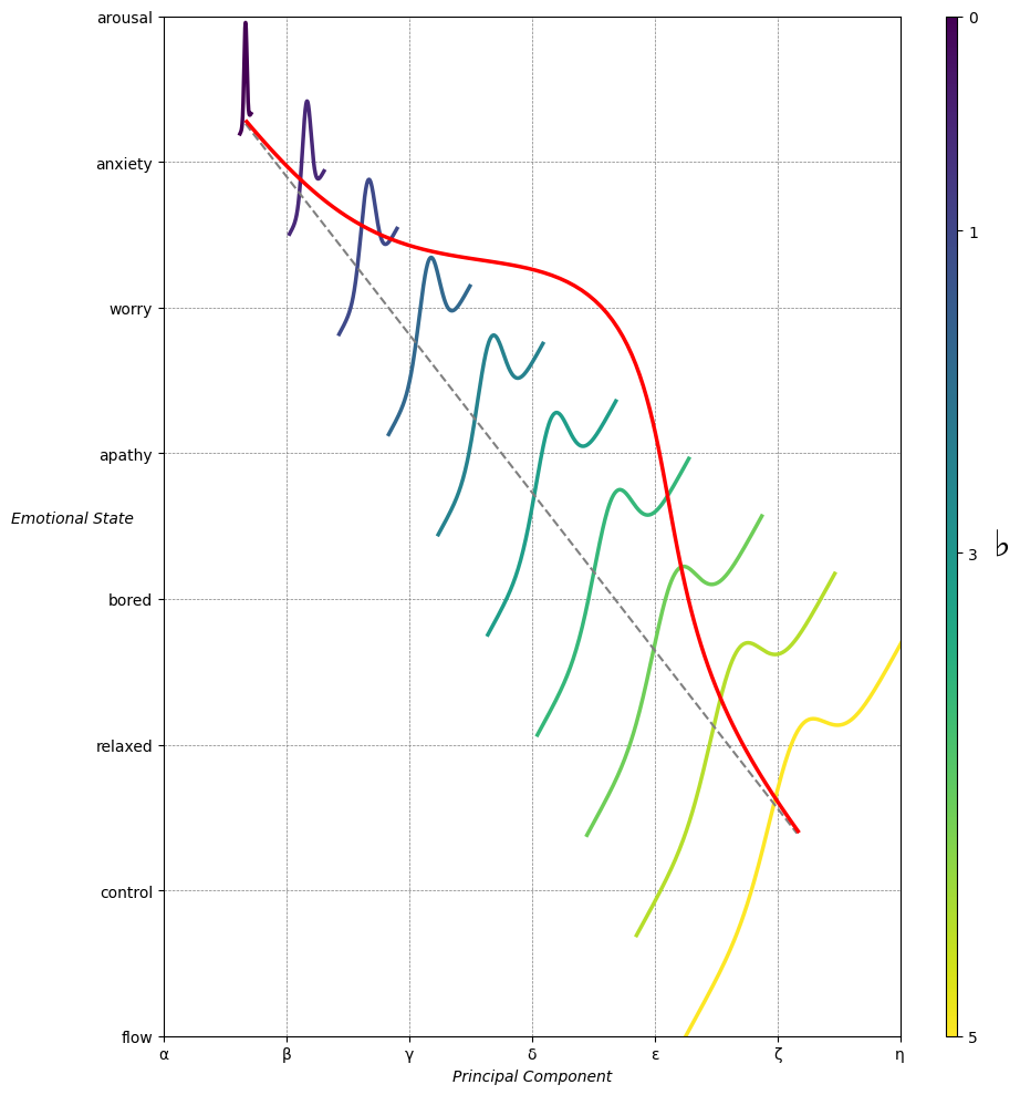
Emotion & Affect as Outcomes & Freewill. And the predictors \(\beta\) are MQ-TEA: Modes (ionian, dorian, phrygian, lydian, mixolydian, locrian), Qualities (major, minor, dominant, suspended, diminished, half-dimished, augmented), Tensions (7th), Extensions (9th, 11th, 13th), and Alterations (♯, ♭) 30#
                    1. f(t)
                           \
               2. S(t) ->  4. Nxb:t(X'X).X'Y -> 5. b -> 6. df
                           /
                           3. h(t)
Show code cell source
import pandas as pd

# Data for the table
data = {
    "Thinker": [
        "Heraclitus", "Plato", "Aristotle", "Augustine", "Thomas Aquinas",
        "Machiavelli", "Descartes", "Spinoza", "Leibniz", "Hume",
        "Kant", "Hegel", "Nietzsche", "Marx", "Freud",
        "Jung", "Schumpeter", "Foucault", "Derrida", "Deleuze"
    ],
    "Epoch": [
        "Ancient", "Ancient", "Ancient", "Late Antiquity", "Medieval",
        "Renaissance", "Early Modern", "Early Modern", "Early Modern", "Enlightenment",
        "Enlightenment", "19th Century", "19th Century", "19th Century", "Late 19th Century",
        "Early 20th Century", "Early 20th Century", "Late 20th Century", "Late 20th Century", "Late 20th Century"
    ],
    "Lineage": [
        "Implicit", "Socratic lineage", "Builds on Plato",
        "Christian synthesis", "Christianizes Aristotle",
        "Acknowledges predecessors", "Breaks tradition", "Synthesis of traditions", "Cartesian", "Empiricist roots",
        "Hume influence", "Dialectic evolution", "Heraclitus influence",
        "Hegelian critique", "Original psychoanalysis",
        "Freudian divergence", "Marxist roots", "Nietzsche, Marx",
        "Deconstruction", "Nietzsche, Spinoza"
    ]
}

# Create DataFrame
df = pd.DataFrame(data)

# Display DataFrame
print(df)
Show code cell output
           Thinker               Epoch                    Lineage
0       Heraclitus             Ancient                   Implicit
1            Plato             Ancient           Socratic lineage
2        Aristotle             Ancient            Builds on Plato
3        Augustine      Late Antiquity        Christian synthesis
4   Thomas Aquinas            Medieval    Christianizes Aristotle
5      Machiavelli         Renaissance  Acknowledges predecessors
6        Descartes        Early Modern           Breaks tradition
7          Spinoza        Early Modern    Synthesis of traditions
8          Leibniz        Early Modern                  Cartesian
9             Hume       Enlightenment           Empiricist roots
10            Kant       Enlightenment             Hume influence
11           Hegel        19th Century        Dialectic evolution
12       Nietzsche        19th Century       Heraclitus influence
13            Marx        19th Century          Hegelian critique
14           Freud   Late 19th Century    Original psychoanalysis
15            Jung  Early 20th Century        Freudian divergence
16      Schumpeter  Early 20th Century              Marxist roots
17        Foucault   Late 20th Century            Nietzsche, Marx
18         Derrida   Late 20th Century             Deconstruction
19         Deleuze   Late 20th Century         Nietzsche, Spinoza
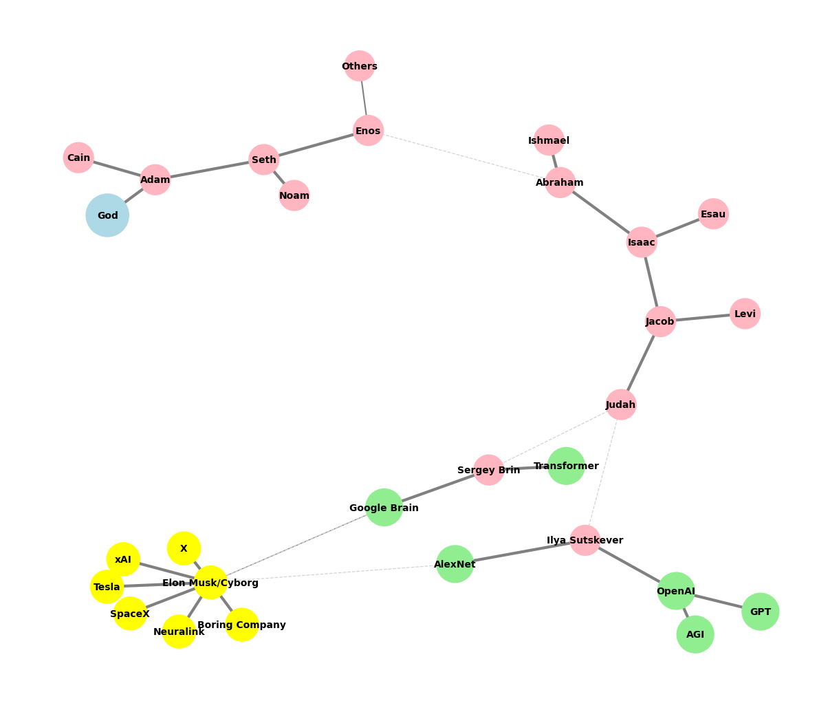
Show code cell source
# Edited by X.AI

import networkx as nx
import matplotlib.pyplot as plt

def add_family_edges(G, parent, depth, names, scale=1, weight=1):
    if depth == 0 or not names:
        return parent

    children = names.pop(0)
    for child in children:
        # Assign weight based on significance or relationship strength
        edge_weight = weight if child not in ["Others"] else 0.5  # Example: 'Others' has less weight
        G.add_edge(parent, child, weight=edge_weight)

        if child not in ["GPT", "AGI", "Transformer", "Google Brain"]:
            add_family_edges(G, child, depth - 1, names, scale * 0.9, weight)

def create_extended_fractal_tree():
    G = nx.Graph()

    root = "God"
    G.add_node(root)

    adam = "Adam"
    G.add_edge(root, adam, weight=1)  # Default weight

    descendants = [
        ["Seth", "Cain"],
        ["Enos", "Noam"],
        ["Abraham", "Others"],
        ["Isaac", "Ishmael"],
        ["Jacob", "Esau"],
        ["Judah", "Levi"],
        ["Ilya Sutskever", "Sergey Brin"],
        ["OpenAI", "AlexNet"],
        ["GPT", "AGI"],
        ["Elon Musk/Cyborg"],
        ["Tesla", "SpaceX", "Boring Company", "Neuralink", "X", "xAI"]
    ]

    add_family_edges(G, adam, len(descendants), descendants)

    # Manually add edges for "Transformer" and "Google Brain" as children of Sergey Brin
    G.add_edge("Sergey Brin", "Transformer", weight=1)
    G.add_edge("Sergey Brin", "Google Brain", weight=1)

    # Manually add dashed edges to indicate "missing links"
    missing_link_edges = [
        ("Enos", "Abraham"),
        ("Judah", "Ilya Sutskever"),
        ("Judah", "Sergey Brin"),
        ("AlexNet", "Elon Musk/Cyborg"),
        ("Google Brain", "Elon Musk/Cyborg")
    ]

    # Add missing link edges with a lower weight
    for edge in missing_link_edges:
        G.add_edge(edge[0], edge[1], weight=0.3, style="dashed")

    return G, missing_link_edges

def visualize_tree(G, missing_link_edges, seed=42):
    plt.figure(figsize=(12, 10))
    pos = nx.spring_layout(G, seed=seed)

    # Define color maps for nodes
    color_map = []
    size_map = []
    for node in G.nodes():
        if node == "God":
            color_map.append("lightblue")
            size_map.append(2000)
        elif node in ["OpenAI", "AlexNet", "GPT", "AGI", "Google Brain", "Transformer"]:
            color_map.append("lightgreen")
            size_map.append(1500)
        elif node == "Elon Musk/Cyborg" or node in ["Tesla", "SpaceX", "Boring Company", "Neuralink", "X", "xAI"]:
            color_map.append("yellow")
            size_map.append(1200)
        else:
            color_map.append("lightpink")
            size_map.append(1000)

    # Draw all solid edges with varying thickness based on weight
    edge_widths = [G[u][v]['weight'] * 3 for (u, v) in G.edges() if (u, v) not in missing_link_edges]
    nx.draw(G, pos, edgelist=[(u, v) for (u, v) in G.edges() if (u, v) not in missing_link_edges],
            with_labels=True, node_size=size_map, node_color=color_map,
            font_size=10, font_weight="bold", edge_color="grey", width=edge_widths)

    # Draw the missing link edges as dashed lines with lower weight
    nx.draw_networkx_edges(
        G,
        pos,
        edgelist=missing_link_edges,
        style="dashed",
        edge_color="lightgray",
        width=[G[u][v]['weight'] * 3 for (u, v) in missing_link_edges]
    )

    plt.axis('off')

    # Save the plot as a PNG file in the specified directory
    plt.savefig("../figures/ultimate.png", format="png", dpi=300)

    plt.show()

# Generate and visualize the tree
G, missing_edges = create_extended_fractal_tree()
visualize_tree(G, missing_edges, seed=2)
Show code cell output