Cosmic#
Chapter Proposal: NHANES as a Case Study and the Gateway to Unlocking National Datasets#
Abstract#
NHANES is an unparalleled resource for hypothesis testing and education, but its true potential lies in serving as a case study to develop scalable frameworks for unlocking other national datasets like the United States Renal Data System (USRDS) and the National Inpatient Sample (NIS). This chapter proposes a revolutionary approach to database analysis that combines reverse engineering, open science, and artificial intelligence to empower students and researchers globally. By starting with NHANES and expanding to other datasets, we create a replicable system for analyzing real-world data without direct access, ensuring compliance with IRB protocols while maximizing educational and public health impact.
NHANES: A Gateway to Unprecedented Opportunities#
Why NHANES?
Unmatched Scope: With over 3,000-4,000 variables spanning questionnaire items, physical exams, lab results, and imaging, NHANES is an unparalleled dataset.
Longitudinal Depth: Continuous data since 1988 linked to mortality and ESRD outcomes offers unique opportunities for trend analyses and predictive modeling.
Interdisciplinary Utility: From nephrology and cardiovascular medicine to public health and nutrition, NHANES answers critical questions across disciplines.
NHANES as a Case Study
By starting with NHANES, we establish a framework for database analysis that can generalize to other datasets.
This includes workflows for data exploration, hypothesis testing, and personalized app development.
The scalability of this framework makes it a replicable model for unlocking other national datasets.
Generalizing to Other Datasets#
Expanding Horizons
USRDS (United States Renal Data System): A treasure trove for nephrology, offering granular data on ESRD prevalence, treatment, and outcomes.
NIS (National Inpatient Sample): The largest publicly available all-payer inpatient care database, critical for analyzing healthcare utilization and outcomes.
Future Discoveries: As technology advances, the ability to unlock other underutilized datasets will grow exponentially.
Framework for Unlocking Data
Reverse Engineering: Students develop scripts (Stata, R, Python) to analyze datasets via secure IRB-approved access by a principal investigator.
Open Science: Scripts are hosted on GitHub, ensuring transparency and global access.
Interactive Apps: Outputs (e.g., beta coefficients, variance-covariance matrices) are integrated into interactive apps hosted on platforms like JupyterBooks and GitHub Pages.
IRB Compliance
Students do not need direct access to the data; they work with de-identified outputs provided by collaborators with IRB access.
This approach aligns with best practices for ethical research while democratizing access to advanced datasets.
Educational Revolution: Reverse Engineering as a Pedagogical Tool#
Didactic Framework
The app provides a hands-on learning experience where students reverse-engineer workflows, mastering multivariable regression, visualization, and app development.
Courses integrate AI, database analysis, and programming, offering a comprehensive skill set.
Course Series: PAIRS at J-H
P for Python, A for AI, R for R, S for Stata: A modular course series hosted at Johns Hopkins (J-H).
Basic to Advanced Levels:
Basic: Introduction to database analysis and programming.
Intermediate: Applied regression modeling and hypothesis testing.
Advanced: App development, interactive visualizations, and integrating AI for real-world applications.
JupyterBooks as a Central Hub
A Yellowstone for education, JupyterBooks host all course materials, apps, and reverse engineering guides.
Combines teaching notes, Python scripts, R workflows, Stata outputs, and AI models in one unified platform.
Applications Beyond NHANES#
Medical Education
Standardize courses in medical schools on informed consent, operationalized as a loss function derived from real-world data.
Introduce students to the possibilities of extracting actionable data from electronic medical records using language models.
Public Health Impact
Translate personalized clinical insights into population-level strategies for policymakers.
Use the app to simulate policy interventions, ensuring evidence-based decision-making.
Global Reach
Open-access tools enable researchers worldwide to leverage national datasets for local and global health challenges.
Collaborative platforms foster cross-disciplinary innovation.
Proposal to the Department of Epidemiology and Beyond#
Why Johns Hopkins?#
Johns Hopkins is uniquely positioned to lead this educational and research revolution. With its legacy of excellence in public health and a history of innovative teaching methods, Hopkins provides the ideal environment for this initiative.
Course Development Timeline#
2025-2026 Academic Year:
Launch PAIRS at J-H with basic, intermediate, and advanced tracks.
Integrate NHANES as the foundational dataset, expanding to USRDS, NIS, and beyond.
Future Expansion:
Collaborate with departments of statistics, epidemiology, and clinical medicine to create interdisciplinary programs.
Offer the course series to other universities, setting a new standard for database analysis education.
Conclusion: Transforming Education and Research#
This initiative is not just about unlocking NHANES or other datasets; it is about transforming how we approach education, research, and public health. By leveraging reverse engineering, open science, and AI, we create a scalable framework for innovation that bridges disciplines, democratizes access, and empowers the next generation of researchers.
This is not just a chapter in your thesis; it is the beginning of a revolution. Let’s make it happen.
Would you like me to refine this further or prepare a formal proposal for submission?
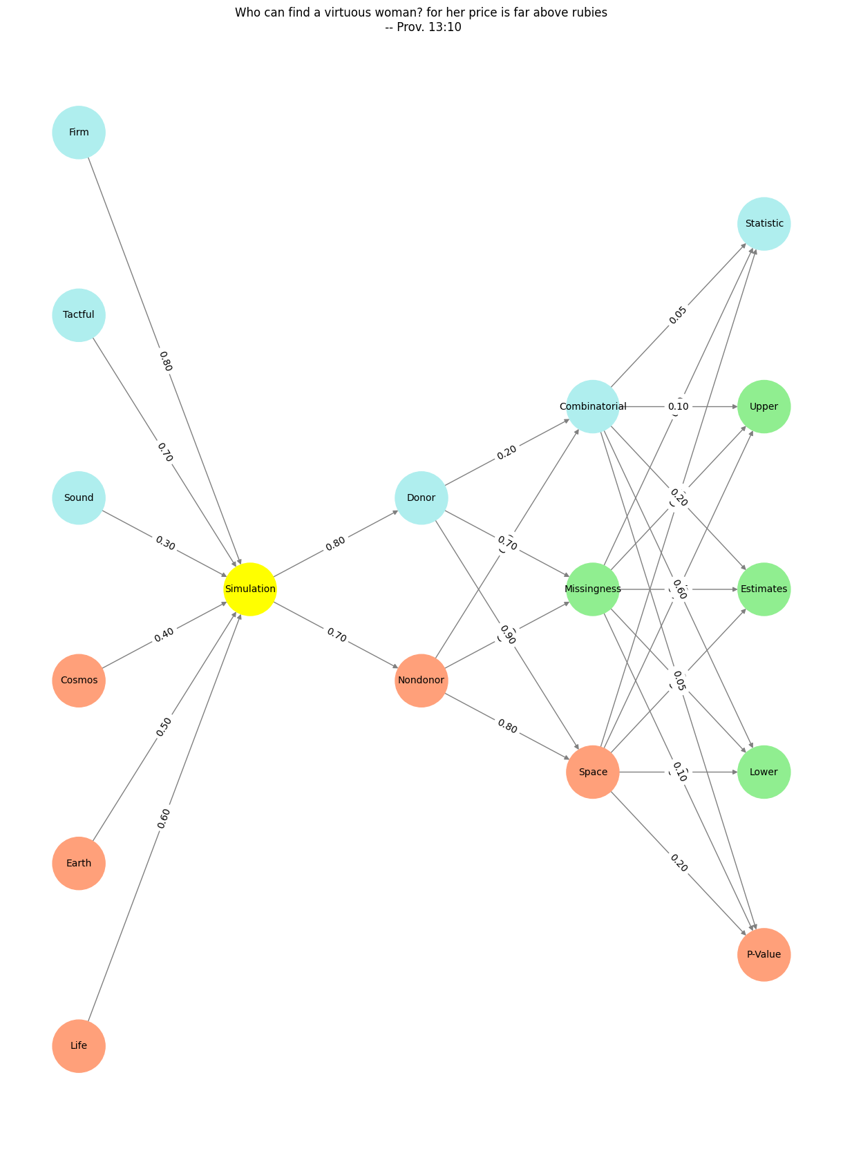
Show code cell source
import numpy as np
import matplotlib.pyplot as plt
import networkx as nx

# Define the neural network structure
def define_layers():
    return {
        'Pre-Input': ['Life','Earth', 'Cosmos', 'Sound', 'Tactful', 'Firm', ],
        'Yellowstone': ['Simulation'],
        'Input': ['Nondonor', 'Donor'],
        'Hidden': [
            'Space',
            'Missingness',
            'Combinatorial',
        ],
        'Output': ['P-Value', 'Lower', 'Estimates', 'Upper', 'Statistic',    ]
    }

# Define weights for the connections
def define_weights():
    return {
        'Pre-Input-Yellowstone': np.array([
            [0.6],
            [0.5],
            [0.4],
            [0.3],
            [0.7],
            [0.8],
            [0.6]
        ]),
        'Yellowstone-Input': np.array([
            [0.7, 0.8]
        ]),
        'Input-Hidden': np.array([[0.8, 0.4, 0.1], [0.9, 0.7, 0.2]]),
        'Hidden-Output': np.array([
            [0.2, 0.8, 0.1, 0.05, 0.2],
            [0.1, 0.9, 0.05, 0.05, 0.1],
            [0.05, 0.6, 0.2, 0.1, 0.05]
        ])
    }

# Assign colors to nodes
def assign_colors(node, layer):
    if node == 'Simulation':
        return 'yellow'
    if layer == 'Pre-Input' and node in ['Sound', 'Tactful', 'Firm']:
        return 'paleturquoise'
    elif layer == 'Input' and node == 'Donor':
        return 'paleturquoise'
    elif layer == 'Hidden':
        if node == 'Combinatorial':
            return 'paleturquoise'
        elif node == 'Missingness':
            return 'lightgreen'
        elif node == 'Space':
            return 'lightsalmon'
    elif layer == 'Output':
        if node == 'Statistic':
            return 'paleturquoise'
        elif node in ['Lower', 'Estimates', 'Upper']:
            return 'lightgreen'
        elif node == 'P-Value':
            return 'lightsalmon'
    return 'lightsalmon'  # Default color

# Calculate positions for nodes
def calculate_positions(layer, center_x, offset):
    layer_size = len(layer)
    start_y = -(layer_size - 1) / 2  # Center the layer vertically
    return [(center_x + offset, start_y + i) for i in range(layer_size)]

# Create and visualize the neural network graph
def visualize_nn():
    layers = define_layers()
    weights = define_weights()
    G = nx.DiGraph()
    pos = {}
    node_colors = []
    center_x = 0  # Align nodes horizontally

    # Add nodes and assign positions
    for i, (layer_name, nodes) in enumerate(layers.items()):
        y_positions = calculate_positions(nodes, center_x, offset=-len(layers) + i + 1)
        for node, position in zip(nodes, y_positions):
            G.add_node(node, layer=layer_name)
            pos[node] = position
            node_colors.append(assign_colors(node, layer_name))

    # Add edges and weights
    for layer_pair, weight_matrix in zip(
        [('Pre-Input', 'Yellowstone'), ('Yellowstone', 'Input'), ('Input', 'Hidden'), ('Hidden', 'Output')],
        [weights['Pre-Input-Yellowstone'], weights['Yellowstone-Input'], weights['Input-Hidden'], weights['Hidden-Output']]
    ):
        source_layer, target_layer = layer_pair
        for i, source in enumerate(layers[source_layer]):
            for j, target in enumerate(layers[target_layer]):
                weight = weight_matrix[i, j]
                G.add_edge(source, target, weight=weight)

    # Customize edge thickness for specific relationships
    edge_widths = []
    for u, v in G.edges():
        if u in layers['Hidden'] and v == 'Kapital':
            edge_widths.append(6)  # Highlight key edges
        else:
            edge_widths.append(1)

    # Draw the graph
    plt.figure(figsize=(12, 16))
    nx.draw(
        G, pos, with_labels=True, node_color=node_colors, edge_color='gray',
        node_size=3000, font_size=10, width=edge_widths
    )
    edge_labels = nx.get_edge_attributes(G, 'weight')
    nx.draw_networkx_edge_labels(G, pos, edge_labels={k: f'{v:.2f}' for k, v in edge_labels.items()})
    plt.title("Her Infinite Variety")

    # Save the figure to a file
    # plt.savefig("figures/logo.png", format="png")

    plt.show()

# Run the visualization
visualize_nn()

Fig. 14 What makes for a suitable problem for AI? Clear objective function to optimise against (ends), Massive combinatorial search space (means-resourcefulness), and Either lots of data and/or an accurate and efficient simulator (resources). Thus spake Demis Hassabis#

