Tactical

Compute Unified Device Architecture (CUDA) enables parallel processing by leveraging GPUs, and its structure is deeply analogous to the concept of exploring a vast combinatorial space to compress time. GPUs are designed to handle thousands of threads simultaneously, much like simulating multiple “universes” or branches of possibilities in parallel rather than sequentially.

In this sense, CUDA’s parallel processing works like a multiverse of computation. Each thread represents an independent timeline, exploring a subset of the combinatorial space. This setup is especially effective for problems where solutions are distributed across a massive number of possibilities, such as:

• Protein folding (AlphaFold): Threads simulate different folding pathways simultaneously, vastly compressing the time to find optimal structures.

• Machine learning: Neural networks train faster because CUDA allows simultaneous calculations for each node’s input, weight, and gradient updates.

• Physics simulations: CUDA can process the behavior of millions of particles or systems at once, akin to running multiple universes to predict a collective outcome.

This parallelism mirrors the philosophical idea of simultaneous “universes,” where each computation evolves independently but contributes to a singular, cohesive output. It’s the ultimate strategy for compressing time: exploring all plausible configurations in the combinatorial space at once instead of linearly traversing them.

The centrality of “Error” in “GenerativeAI” aligns with the idea that progress arises from iterative failures—a Nietzschean will-to-power disguised as trial and error.

CUDA, in essence, doesn’t just simulate the many worlds—it enables us to harvest insights from them simultaneously. This makes it an extraordinary metaphor for how modern computational systems, from AI to astrophysics, are increasingly mirroring the complexity of the universe itself.

Show code cell source Hide code cell source

import numpy as np
import matplotlib.pyplot as plt
import networkx as nx

# Define the neural network structure; modified to align with "Aprés Moi, Le Déluge" (i.e. Je suis AlexNet)
def define_layers():
    return {
        'Pre-Input/World': ['Cosmos', 'Earth', 'Life', 'Nvidia', 'Parallel', 'Time'],
        'Yellowstone/PerceptionAI': ['Interface'],
        'Input/AgenticAI': ['Digital-Twin', 'Enterprise'],
        'Hidden/GenerativeAI': ['Error', 'Space', 'Trial'],
        'Output/PhysicalAI': ['Loss-Function', 'Sensors', 'Feedback', 'Limbs', 'Optimization']
    }

# Assign colors to nodes
def assign_colors(node, layer):
    if node == 'Interface':
        return 'yellow'
    if layer == 'Pre-Input/World' and node in [ 'Time']:
        return 'paleturquoise'
    if layer == 'Pre-Input/World' and node in [ 'Parallel']:
        return 'lightgreen'
    elif layer == 'Input/AgenticAI' and node == 'Enterprise':
        return 'paleturquoise'
    elif layer == 'Hidden/GenerativeAI':
        if node == 'Trial':
            return 'paleturquoise'
        elif node == 'Space':
            return 'lightgreen'
        elif node == 'Error':
            return 'lightsalmon'
    elif layer == 'Output/PhysicalAI':
        if node == 'Optimization':
            return 'paleturquoise'
        elif node in ['Limbs', 'Feedback', 'Sensors']:
            return 'lightgreen'
        elif node == 'Loss-Function':
            return 'lightsalmon'
    return 'lightsalmon'  # Default color

# Calculate positions for nodes
def calculate_positions(layer, center_x, offset):
    layer_size = len(layer)
    start_y = -(layer_size - 1) / 2  # Center the layer vertically
    return [(center_x + offset, start_y + i) for i in range(layer_size)]

# Create and visualize the neural network graph
def visualize_nn():
    layers = define_layers()
    G = nx.DiGraph()
    pos = {}
    node_colors = []
    center_x = 0  # Align nodes horizontally

    # Add nodes and assign positions
    for i, (layer_name, nodes) in enumerate(layers.items()):
        y_positions = calculate_positions(nodes, center_x, offset=-len(layers) + i + 1)
        for node, position in zip(nodes, y_positions):
            G.add_node(node, layer=layer_name)
            pos[node] = position
            node_colors.append(assign_colors(node, layer_name))

    # Add edges (without weights)
    for layer_pair in [
        ('Pre-Input/World', 'Yellowstone/PerceptionAI'), ('Yellowstone/PerceptionAI', 'Input/AgenticAI'), ('Input/AgenticAI', 'Hidden/GenerativeAI'), ('Hidden/GenerativeAI', 'Output/PhysicalAI')
    ]:
        source_layer, target_layer = layer_pair
        for source in layers[source_layer]:
            for target in layers[target_layer]:
                G.add_edge(source, target)

    # Draw the graph
    plt.figure(figsize=(12, 8))
    nx.draw(
        G, pos, with_labels=True, node_color=node_colors, edge_color='gray',
        node_size=3000, font_size=10, connectionstyle="arc3,rad=0.1"
    )
    plt.title("Archimedes", fontsize=15)
    plt.show()

# Run the visualization
visualize_nn()

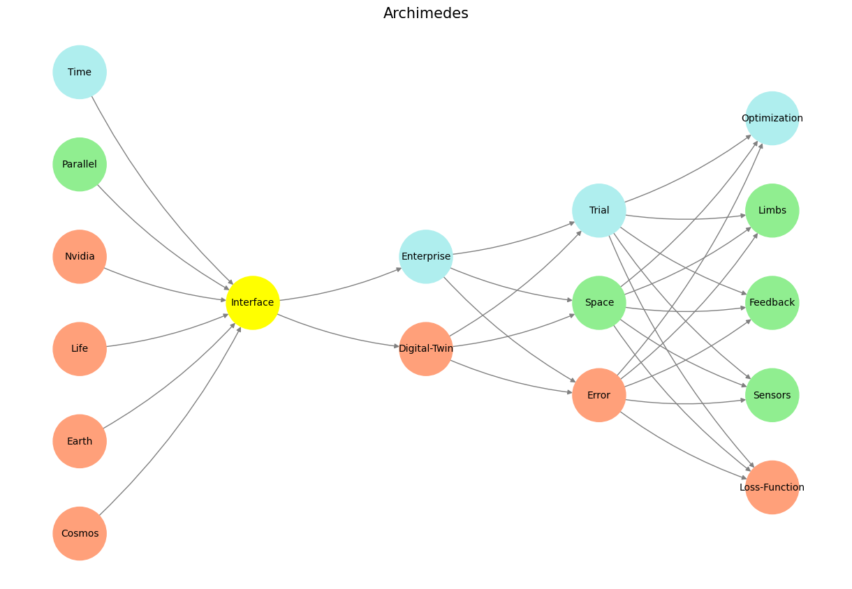
Fig. 1 Time is Money. If the ultimate thing we crave is time (wherein much can be achieved: demand/reward), and that we can produce a vast combinatorial space through wide & deep neural networks (neural network architecture: supply/risk), then parallel processing of various branches in the vast combinatorial space is the means by which time may be compressed. Top tech companies a paying top-dollar to Nvidia, who dominate parallel processing with their GPUs (saving time, saving money, willing to pay: price/resource). see Resource