Woo’d 🗡️❤️💰

Scaling in machine learning—whether pre-training, post-training, or test-time—represents distinct phases of refining and applying models to achieve increasingly sophisticated reasoning. Pre-training scaling focuses on expanding the size of datasets and model architectures before any fine-tuning. In 2025, the human race will generate more data than its ever generated throughout history. And so larger models trained on broader datasets will have more likelihood of acquiring generalized reasoning capabilities, akin to forming a vast foundation of latent knowledge. This stage emphasizes data diversity and model capacity to encode complex patterns and vast combinatorial spaces into an algorithm, thereby setting the stage for downstream adaptability and emergent properties akin to the Red Queen Hypothesis.

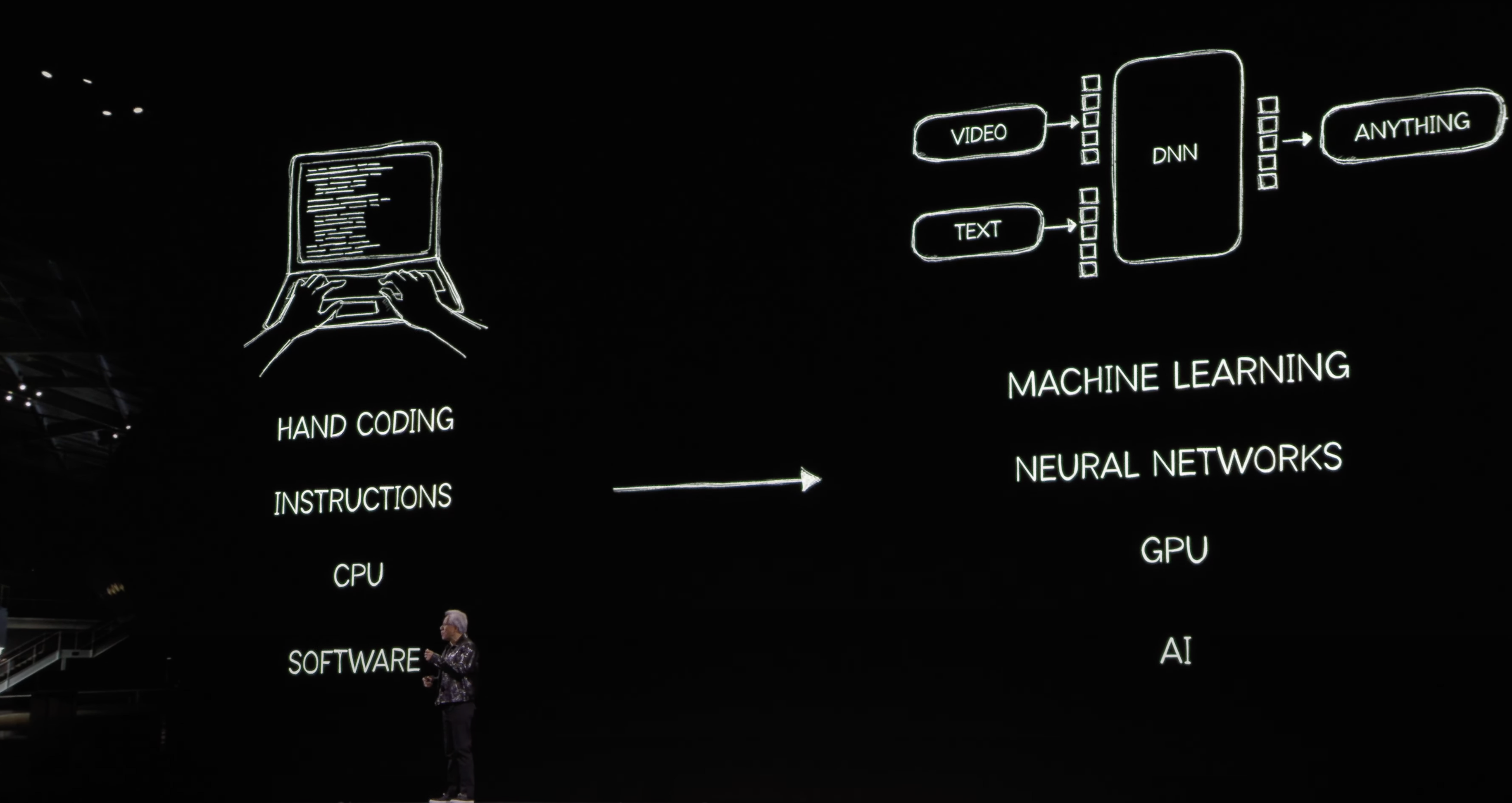
Fig. 6 Google’s 2018 Transformer Was Exactly That. Transformation of inputs (one mode e.g. text) to outputs (another mode e.g. video); i.e., machines learning that vast combinatorial space. All taken together, that is artificial intelligence

Post-training scaling, by contrast, refines the model after pre-training, often involving fine-tuning on domain-specific datasets or augmenting the architecture with additional parameters. It prioritizes specialization, narrowing the focus of the model to align with specific tasks while leveraging the robust baseline reasoning capabilities established during pre-training. This phase can be seen as sharpening a multi-purpose tool into a finely-tuned instrument (e.g. reinforcement learning through human feedback). This mostly has to do with alignment with value systems rather than efficiency.

Show code cell source Hide code cell source

import numpy as np
import matplotlib.pyplot as plt
import networkx as nx

# Define the neural network structure; modified to align with "Aprés Moi, Le Déluge" (i.e. Je suis AlexNet)
def define_layers():
    return {
        'Pre-Input/CudAlexnet': ['Life', 'Earth', 'Cosmos', 'Sound', 'Tactful', 'Firm'],
        'Yellowstone/SensoryAI': ['G1 & G2'],
        'Input/AgenticAI': ['N4, N5', 'N1, N2, N3'],
        'Hidden/GenerativeAI': ['Sympathetic', 'G3', 'Parasympathetic'],
        'Output/PhysicalAI': ['Ecosystem', 'Vulnerabilities', 'AChR', 'Strengths', 'Neurons']
    }

# Assign colors to nodes
def assign_colors(node, layer):
    if node == 'G1 & G2':
        return 'yellow'
    if layer == 'Pre-Input/CudAlexnet' and node in ['Sound', 'Tactful', 'Firm']:
        return 'paleturquoise'
    elif layer == 'Input/AgenticAI' and node == 'N1, N2, N3':
        return 'paleturquoise'
    elif layer == 'Hidden/GenerativeAI':
        if node == 'Parasympathetic':
            return 'paleturquoise'
        elif node == 'G3':
            return 'lightgreen'
        elif node == 'Sympathetic':
            return 'lightsalmon'
    elif layer == 'Output/PhysicalAI':
        if node == 'Neurons':
            return 'paleturquoise'
        elif node in ['Strengths', 'AChR', 'Vulnerabilities']:
            return 'lightgreen'
        elif node == 'Ecosystem':
            return 'lightsalmon'
    return 'lightsalmon'  # Default color

# Calculate positions for nodes
def calculate_positions(layer, center_x, offset):
    layer_size = len(layer)
    start_y = -(layer_size - 1) / 2  # Center the layer vertically
    return [(center_x + offset, start_y + i) for i in range(layer_size)]

# Create and visualize the neural network graph
def visualize_nn():
    layers = define_layers()
    G = nx.DiGraph()
    pos = {}
    node_colors = []
    center_x = 0  # Align nodes horizontally

    # Add nodes and assign positions
    for i, (layer_name, nodes) in enumerate(layers.items()):
        y_positions = calculate_positions(nodes, center_x, offset=-len(layers) + i + 1)
        for node, position in zip(nodes, y_positions):
            G.add_node(node, layer=layer_name)
            pos[node] = position
            node_colors.append(assign_colors(node, layer_name))

    # Add edges (without weights)
    for layer_pair in [
        ('Pre-Input/CudAlexnet', 'Yellowstone/SensoryAI'), ('Yellowstone/SensoryAI', 'Input/AgenticAI'), ('Input/AgenticAI', 'Hidden/GenerativeAI'), ('Hidden/GenerativeAI', 'Output/PhysicalAI')
    ]:
        source_layer, target_layer = layer_pair
        for source in layers[source_layer]:
            for target in layers[target_layer]:
                G.add_edge(source, target)

    # Draw the graph
    plt.figure(figsize=(12, 8))
    nx.draw(
        G, pos, with_labels=True, node_color=node_colors, edge_color='gray',
        node_size=3000, font_size=10, connectionstyle="arc3,rad=0.1"
    )
    plt.title("Red Queen Hypothesis", fontsize=15)
    plt.show()

# Run the visualization
visualize_nn()

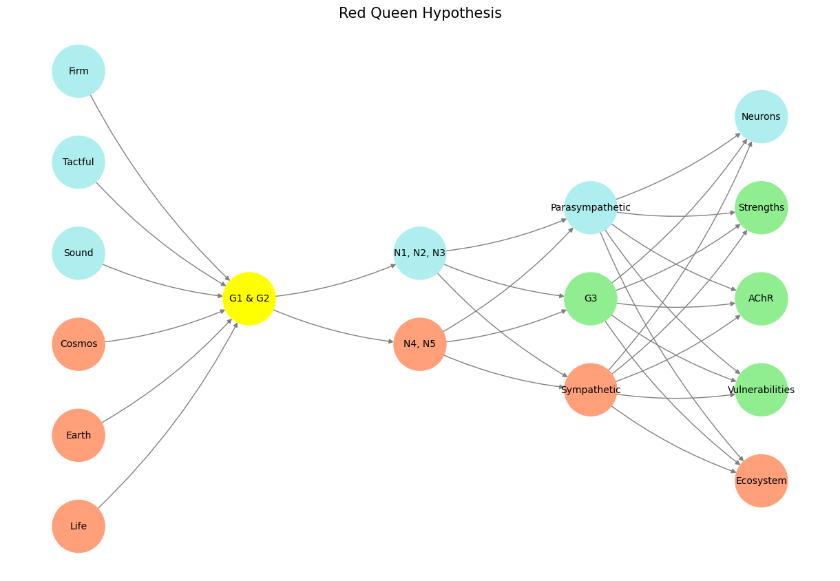
Fig. 7 Cambridge University Graduates. They transplanted their notions of the sound means of tradition, the justified tactics of change within stability, and firm and resolute commitment to share ideals of humanity. And setup the stage for an aburd scene in Athens – A Midsummer Nights Dream

Finally, test-time scaling pertains to the dynamic adjustments made while the model is deployed, including techniques like ensemble methods or prompting strategies. These methods optimize the model’s reasoning on-the-fly, enhancing performance without altering underlying weights. Test-time scaling exemplifies situational adaptability, allowing models to perform better under variable conditions or with constrained resources. Together, these three scaling dimensions create a lifecycle of learning that evolves from general capability to specialized application and adaptive execution, mirroring human reasoning from foundational learning to expert decision-making in real-world scenarios.