
Born to Etiquette#
The expression “(exposome + transcriptome)/genome” offers a compact yet intriguing framework for understanding the interplay between variability and stability in biological systems. At its core, it juxtaposes the chaotic, error-prone nature of somatic processes against the more stable, inherited foundation of the germline. The “noise” component, tied to somatic cells, reflects the imperfections and unpredictability that arise during an organism’s lifetime. Replication errors in the transcriptome—the dynamic set of RNA molecules transcribed from DNA—introduce variability as cells divide and function. These errors, though often small, can accumulate, altering how genes are expressed and potentially leading to dysfunction. Layered onto this is the “exposome,” a term encapsulating the totality of environmental exposures an organism encounters, from chemicals to radiation to lifestyle factors. Mutations driven by the exposome further amplify this noise, embedding external influences into the somatic landscape and pushing it further from its original blueprint.

Fig. 34 In the beginning was the word. And the word was with God. And the word was God. Language is what distinguishes man from all other mammals. Every elaboration of our metaphysics including physics itself is inconceivable without the richness of our languages. It should come as no surprise, then, that LLMs are the mode of AI that transformed this industry beyond promise to .. cadence?#
In contrast, the “signal” of the germline represents a clearer, more reliable transmission of information across generations. Anchored in the genome—the hereditary DNA sequence—it embodies stability and continuity. The germline’s role is to preserve the integrity of genetic instructions, passing them down with remarkable fidelity despite the noise that somatic cells endure. This dichotomy between noise and signal mirrors a fundamental tension in biology: the somatic realm is where adaptation, aging, and disease play out, while the germline safeguards the species’ evolutionary trajectory. The equation-like structure of the expression suggests a ratio or balance, hinting that the noise of somatic changes exists in constant dialogue with the signal of germline inheritance, each shaping the other in subtle ways.
Philosophically, this framework invites reflection on the nature of life itself—how much of it is defined by the pristine signal of our origins, and how much is sculpted by the noisy deviations of lived experience. Scientifically, it aligns with modern understandings of cancer, aging, and epigenetics, where somatic mutations and environmental factors disrupt the harmony of cellular function, often in contrast to the germline’s relative constancy. The use of terms like “transcriptome” and “exposome” grounds the expression in cutting-edge biological thought, while its abstract form encourages interpretation. It’s a poetic shorthand for a complex reality, blending precision with ambiguity to provoke deeper inquiry into the forces that govern life’s continuity and change.
Show code cell source
import numpy as np
import matplotlib.pyplot as plt
import networkx as nx

# Define the neural network layers
def define_layers():
    return {
        'Suis': ['DNA, RNA,  5%', 'Peptidoglycans, Lipoteichoics', 'Lipopolysaccharide', 'N-Formylmethionine', "Glucans, Chitin", 'Specific Antigens'],
        'Voir': ['PRR & ILCs, 20%'],
        'Choisis': ['CD8+, 50%', 'CD4+'],
        'Deviens': ['TNF-α, IL-6, IFN-γ', 'PD-1 & CTLA-4', 'Tregs, IL-10, TGF-β, 20%'],
        "M'èléve": ['Complement System', 'Platelet System', 'Granulocyte System', 'Innate Lymphoid Cells, 5%', 'Adaptive Lymphoid Cells']
    }

# Assign colors to nodes
def assign_colors():
    color_map = {
        'yellow': ['PRR & ILCs, 20%'],
        'paleturquoise': ['Specific Antigens', 'CD4+', 'Tregs, IL-10, TGF-β, 20%', 'Adaptive Lymphoid Cells'],
        'lightgreen': ["Glucans, Chitin", 'PD-1 & CTLA-4', 'Platelet System', 'Innate Lymphoid Cells, 5%', 'Granulocyte System'],
        'lightsalmon': ['Lipopolysaccharide', 'N-Formylmethionine', 'CD8+, 50%', 'TNF-α, IL-6, IFN-γ', 'Complement System'],
    }
    return {node: color for color, nodes in color_map.items() for node in nodes}

# Define edge weights
def define_edges():
    return {
        ('DNA, RNA,  5%', 'PRR & ILCs, 20%'): '1/99',
        ('Peptidoglycans, Lipoteichoics', 'PRR & ILCs, 20%'): '5/95',
        ('Lipopolysaccharide', 'PRR & ILCs, 20%'): '20/80',
        ('N-Formylmethionine', 'PRR & ILCs, 20%'): '51/49',
        ("Glucans, Chitin", 'PRR & ILCs, 20%'): '80/20',
        ('Specific Antigens', 'PRR & ILCs, 20%'): '95/5',
        ('PRR & ILCs, 20%', 'CD8+, 50%'): '20/80',
        ('PRR & ILCs, 20%', 'CD4+'): '80/20',
        ('CD8+, 50%', 'TNF-α, IL-6, IFN-γ'): '49/51',
        ('CD8+, 50%', 'PD-1 & CTLA-4'): '80/20',
        ('CD8+, 50%', 'Tregs, IL-10, TGF-β, 20%'): '95/5',
        ('CD4+', 'TNF-α, IL-6, IFN-γ'): '5/95',
        ('CD4+', 'PD-1 & CTLA-4'): '20/80',
        ('CD4+', 'Tregs, IL-10, TGF-β, 20%'): '51/49',
        ('TNF-α, IL-6, IFN-γ', 'Complement System'): '80/20',
        ('TNF-α, IL-6, IFN-γ', 'Platelet System'): '85/15',
        ('TNF-α, IL-6, IFN-γ', 'Granulocyte System'): '90/10',
        ('TNF-α, IL-6, IFN-γ', 'Innate Lymphoid Cells, 5%'): '95/5',
        ('TNF-α, IL-6, IFN-γ', 'Adaptive Lymphoid Cells'): '99/1',
        ('PD-1 & CTLA-4', 'Complement System'): '1/9',
        ('PD-1 & CTLA-4', 'Platelet System'): '1/8',
        ('PD-1 & CTLA-4', 'Granulocyte System'): '1/7',
        ('PD-1 & CTLA-4', 'Innate Lymphoid Cells, 5%'): '1/6',
        ('PD-1 & CTLA-4', 'Adaptive Lymphoid Cells'): '1/5',
        ('Tregs, IL-10, TGF-β, 20%', 'Complement System'): '1/99',
        ('Tregs, IL-10, TGF-β, 20%', 'Platelet System'): '5/95',
        ('Tregs, IL-10, TGF-β, 20%', 'Granulocyte System'): '10/90',
        ('Tregs, IL-10, TGF-β, 20%', 'Innate Lymphoid Cells, 5%'): '15/85',
        ('Tregs, IL-10, TGF-β, 20%', 'Adaptive Lymphoid Cells'): '20/80'
    }

# Define edges to be highlighted in black
def define_black_edges():
    return {
        ('Tregs, IL-10, TGF-β, 20%', 'Complement System'): '1/99',
        ('Tregs, IL-10, TGF-β, 20%', 'Platelet System'): '5/95',
        ('Tregs, IL-10, TGF-β, 20%', 'Granulocyte System'): '10/90',
        ('Tregs, IL-10, TGF-β, 20%', 'Innate Lymphoid Cells, 5%'): '15/85',
        ('Tregs, IL-10, TGF-β, 20%', 'Adaptive Lymphoid Cells'): '20/80'
    }

# Calculate node positions
def calculate_positions(layer, x_offset):
    y_positions = np.linspace(-len(layer) / 2, len(layer) / 2, len(layer))
    return [(x_offset, y) for y in y_positions]

# Create and visualize the neural network graph
def visualize_nn():
    layers = define_layers()
    colors = assign_colors()
    edges = define_edges()
    black_edges = define_black_edges()

    G = nx.DiGraph()
    pos = {}
    node_colors = []

    # Create mapping from original node names to numbered labels
    mapping = {}
    counter = 1
    for layer in layers.values():
        for node in layer:
            mapping[node] = f"{counter}. {node}"
            counter += 1

    # Add nodes with new numbered labels and assign positions
    for i, (layer_name, nodes) in enumerate(layers.items()):
        positions = calculate_positions(nodes, x_offset=i * 2)
        for node, position in zip(nodes, positions):
            new_node = mapping[node]
            G.add_node(new_node, layer=layer_name)
            pos[new_node] = position
            node_colors.append(colors.get(node, 'lightgray'))

    # Add edges with updated node labels
    edge_colors = []
    for (source, target), weight in edges.items():
        if source in mapping and target in mapping:
            new_source = mapping[source]
            new_target = mapping[target]
            G.add_edge(new_source, new_target, weight=weight)
            edge_colors.append('black' if (source, target) in black_edges else 'lightgrey')

    # Draw the graph
    plt.figure(figsize=(12, 8))
    edges_labels = {(u, v): d["weight"] for u, v, d in G.edges(data=True)}

    nx.draw(
        G, pos, with_labels=True, node_color=node_colors, edge_color=edge_colors,
        node_size=3000, font_size=9, connectionstyle="arc3,rad=0.2"
    )
    nx.draw_networkx_edge_labels(G, pos, edge_labels=edges_labels, font_size=8)
    plt.title("OPRAH™: Distributed Network", fontsize=18)
    plt.show()

# Run the visualization
visualize_nn()
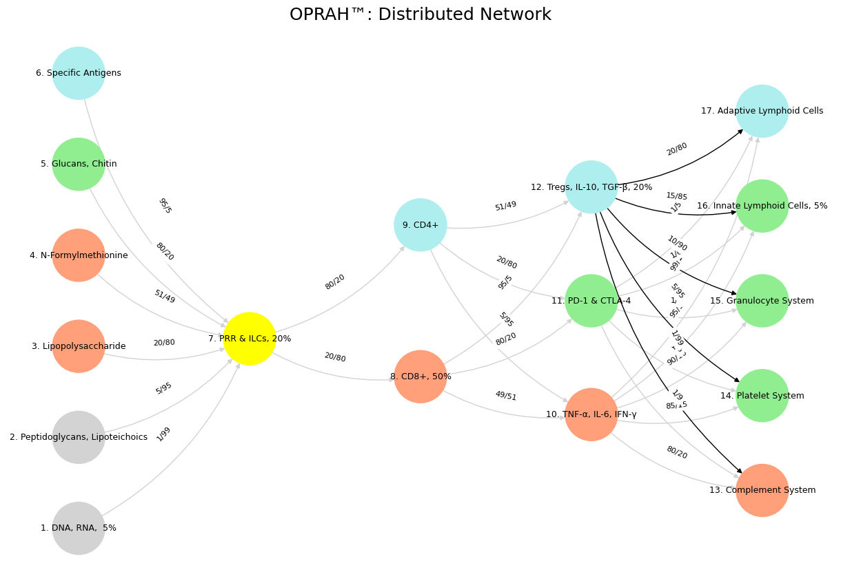
Fig. 35 Glenn Gould and Leonard Bernstein famously disagreed over the tempo and interpretation of Brahms’ First Piano Concerto during a 1962 New York Philharmonic concert, where Bernstein, conducting, publicly distanced himself from Gould’s significantly slower-paced interpretation before the performance began, expressing his disagreement with the unconventional approach while still allowing Gould to perform it as planned; this event is considered one of the most controversial moments in classical music history.#