GPT

                1. f(t)
                      \
           2. S(t) -> 4. y:h'(f)=0;t(X'X).X'Y -> 5. b(c) -> 6. SV'
                      /
                      3. h(t) 

• Text, \(\mu\): Multimodal (beyond text input-token or melody-note)

Show code cell source Hide code cell source

import matplotlib.pyplot as plt
import numpy as np

# Clock settings; f(t) random disturbances making "paradise lost"
clock_face_radius = 1.0
number_of_ticks = 8
tick_labels = [
    "Ionian", "Dorian", "Phrygian", "Lydian",
    "Mixolydian", "Aeolian", "Locrian", "Other"
]

# Calculate the angles for each tick (in radians)
angles = np.linspace(0, 2 * np.pi, number_of_ticks, endpoint=False)
# Inverting the order to make it counterclockwise
angles = angles[::-1]

# Create figure and axis
fig, ax = plt.subplots(figsize=(8, 8))
ax.set_xlim(-1.2, 1.2)
ax.set_ylim(-1.2, 1.2)
ax.set_aspect('equal')

# Draw the clock face
clock_face = plt.Circle((0, 0), clock_face_radius, color='lightgrey', fill=True)
ax.add_patch(clock_face)

# Draw the ticks and labels
for angle, label in zip(angles, tick_labels):
    x = clock_face_radius * np.cos(angle)
    y = clock_face_radius * np.sin(angle)
    
    # Draw the tick
    ax.plot([0, x], [0, y], color='black')
    
    # Positioning the labels slightly outside the clock face
    label_x = 1.1 * clock_face_radius * np.cos(angle)
    label_y = 1.1 * clock_face_radius * np.sin(angle)
    
    # Adjusting label alignment based on its position
    ha = 'center'
    va = 'center'
    if np.cos(angle) > 0:
        ha = 'left'
    elif np.cos(angle) < 0:
        ha = 'right'
    if np.sin(angle) > 0:
        va = 'bottom'
    elif np.sin(angle) < 0:
        va = 'top'
    
    ax.text(label_x, label_y, label, horizontalalignment=ha, verticalalignment=va, fontsize=10)

# Remove axes
ax.axis('off')

# Show the plot
plt.show()

Show code cell output Hide code cell output

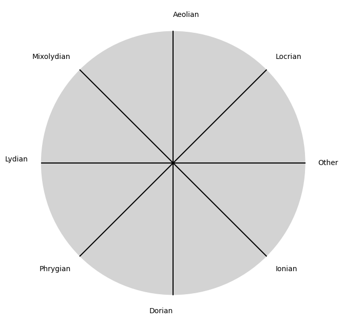
• Contex, \(\sigma\): Better at recognizing patterns across modes (applicable as much to music)

• Pretext, \(\%\): Improved prediction (in music its increased likelihood of marvelling from a familiar ambiguity)

• AM. great music is all about flirtation with “other” modes. While the modes are all within diatonic, the flirtation may borrow a mode from a different tonal center. Bach’s 1068ii, for instance, has an Ionian center on D, but its first flirtation is with the Dorian mode’s bII in bar 5

• GPT. Absolutely! Great music often involves a playful exploration of different modes and tonal centers, creating a rich and complex tapestry of sound. In Bach’s BWV 1068 II (Air), the piece is fundamentally in D major (Ionian mode), which provides a sense of stability and clarity.

• However, in bar 5, Bach introduces a C natural, which is the flattened second (bII) degree in the Dorian mode. This brief departure adds a layer of tension and intrigue, subtly shifting the listener’s expectations. The use of the bII (a note typically outside the Ionian mode of D) momentarily transports the piece into a different emotional and tonal space, creating a beautiful contrast before resolving back to the home key.

• This kind of modal mixture is a hallmark of Bach’s genius. By borrowing from the Dorian mode, he adds depth and variety to the music, making it both intellectually stimulating and emotionally resonant. It’s this interplay between familiar and unexpected elements that keeps listeners engaged and makes Bach’s compositions timeless.

• Do you see similar modal flirtations in other works that you enjoy?

• AM. I’m all Bach for now. Actually, the C natural is correct. It first appears in bar 5, but it’s the II not bII of the dorian. The II of the dorian is F#-A-C

• GPT. You’re absolutely right. In the context of Dorian mode, the II chord would indeed be F#-A-C. Bach’s use of C natural in bar 5 still represents a modal mixture, as it deviates from the pure D major scale. This subtle incorporation enriches the harmonic texture, providing a momentary shift that enhances the overall musical experience.

• Bach’s ability to weave these modal influences seamlessly into his compositions is a testament to his mastery. His work in BWV 1068 II demonstrates a sophisticated understanding of harmony and modal interplay, creating music that is both structurally intricate and deeply expressive.

• It’s fascinating to see how these modal shifts contribute to the emotional and intellectual depth of his music. Would you like to explore more specific examples of modal interplay in Bach’s other works?

\(\mu\) tokens Base-case/Pretraining

• Pre-training: GPT models are pre-trained on a large corpus of text data. During this phase, the model learns the statistical properties of the language, including grammar, vocabulary, idioms, and even some factual knowledge. This pre-training is done in an unsupervised manner, meaning the model doesn’t know the “correct” output; instead, it learns by predicting the next word in a sentence based on the previous words.

• In essence, GPT models are powerful because they can use the context provided by the input data to make informed predictions. The “training context” is all the data and patterns the model has seen during pre-training, and this rich background allows it to generate coherent and contextually appropriate responses. This approach enables the model to handle a wide range of tasks, from language translation to text completion, all while maintaining a contextual awareness that makes its predictions relevant and accurate.

• Similarly, in a Transformer model, the “melody” can be thought of as the input tokens (words, for instance). The “chords” are the surrounding words or tokens that the attention mechanism uses to reinterpret the context of each word. Just as the meaning of the note B changes with different chords, the significance of a word can shift depending on its context provided by other words. The attention mechanism dynamically adjusts the “chordal” context, allowing the model to emphasize different aspects or interpretations of the same input

\(\sigma\) context Varcov-matrix/Transformer

• Contextual Understanding: The training phase helps the model understand context by looking at how words and phrases are used together. This is where the attention mechanism comes into play—it allows the model to focus on different parts of the input data, effectively “learning” the context in which words appear.

\(\%\) meaning Predictive-accuracy/Generative

• Contextual Predictions: Once trained, the model can generate predictions based on the context provided by the input text. For example, if given a sentence, it can predict the next word or complete the sentence by considering the context provided by the preceding words. The model uses the patterns it learned during training to make these predictions, ensuring they are contextually relevant.

• Dynamic Attention: The attention mechanism is key to this process. It allows the model to weigh the importance of different words or tokens in the input, effectively understanding which parts of the context are most relevant to the prediction. This dynamic adjustment is what gives GPT models their flexibility and nuanced understanding.

                     1. Observing
                                \
           2. Time = Compute -> 4. Collective Unconscious -> 5. Decoding -> 6. Generation-Imitation-Prediction-Representation
                                /
                                3. Encoding
  

Show code cell source Hide code cell source

import numpy as np
import matplotlib.pyplot as plt
import scipy.stats as stats

# Parameters for German distribution
N_german = 124038
mean_german = 1387
std_german = 389

# Parameters for FIDE distribution
N_fide = 120725
mean_fide = 2122
std_fide = 182

# Generate x values
x = np.linspace(mean_german - 4*std_german, mean_fide + 4*std_fide, 1000)

# Calculate the t-distributions
density_german = stats.t.pdf(x, df=N_german-1, loc=mean_german, scale=std_german)
density_fide = stats.t.pdf(x, df=N_fide-1, loc=mean_fide, scale=std_fide)

# Plotting the distributions
plt.figure(figsize=(10, 6))
plt.plot(x, density_german, label='German', color='blue')
plt.plot(x, density_fide, label='FIDE', color='red')
plt.fill_between(x, density_german, alpha=0.3, color='blue')
plt.fill_between(x, density_fide, alpha=0.3, color='red')

# Customizing the aesthetics
plt.title('Overlayed t-Distributions: German vs FIDE')
plt.xlabel('Values')
plt.ylabel('Density')
plt.legend()

# Remove the top and right spines
plt.gca().spines['top'].set_visible(False)
plt.gca().spines['right'].set_visible(False)

# Add a very light dotted grid
plt.grid(True, linestyle=':', color='gray', alpha=0.6)

# Show the plot
plt.show()

Show code cell output Hide code cell output

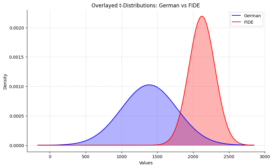
Elo Rating as reported by X.ai@Grok. Distribution of chess skill as measured by Elo rating in FIDE (blue color) and German (red) databases (as of 2008) for reference. The databases contain similar number of players, but differ vastly in the distribution shape and coverage—the only overlap is at the highest values of the German database and lowest values of the FIDE database.