
Anchor ⚓️#
The Neural Framework for Personalized Donor Insights#
The Pre-Input Layer: Foundation of Data-Driven Design#
The pre-input layer serves as the neural network’s connection to reality, integrating raw data with analytical rigor. Here, data such as target populations (donors vs. non-donors), sources, and eligibility criteria form the cornerstone of the model. This is where multivariable regression comes into play, extracting meaningful patterns from this foundational data set. The coefficient vector and the variance-covariance matrix ensure the model reflects not just central tendencies but also the interdependencies and uncertainties inherent in donor and non-donor comparisons. Together, these components ensure that every output is rooted in robust, evidence-based computation.
The Yellowstone Node (G1 & G2): The Backend Ecosystem#
At the heart of the app’s functionality lies the Yellowstone node, which corresponds to the JavaScript and HTML backbone of our platform. Like the ecological impact of wolves reintroduced into Yellowstone National Park, this layer drives cascading effects throughout the system. The backend ensures seamless data processing and visualization, enabling the end-user to interact with a complex yet intuitive interface. This is the engine that transforms raw pre-input data into actionable insights.
Input Layer (N1-N5): Defining Patient Parameters#
The input layer, represented by N1-N5, captures the patient population parameters selected by the end-user. These nodes enable granular control over study vs. control group definitions, with each node symbolizing a vital characteristic:
N1-N3: Factors distinguishing donors (e.g., age, BMI, medical history).
N4-N5: Parameters related to control populations (e.g., non-donors of similar demographics).
By allowing these customizable inputs, the app ensures that personalized risk assessments remain contextually grounded, reflecting the nuances of each unique case.
The Output Layer: Personalized Risk and Precision#
The output layer delivers the model’s ultimate goal: personalized risk estimates and their standard errors. These outputs are optimized for clarity and relevance, ensuring that end-users can make well-informed decisions. Each output is a synthesis of:
Ecosystemic Impact: The broader implications of kidney donation on both individual health and healthcare systems.
Vulnerabilities: Identification of potential risks tailored to the donor’s profile.
Strengths: Highlighting areas of resilience and compatibility for donation.
AChR (Acetylcholine Receptor Analogy): A focus on key decision-making thresholds, akin to ligand-receptor interactions.
A Novel Approach to Informed Consent#
Traditionally, informed consent has been a qualitative endeavor, reliant on subjective understanding. In our model, we redefine informed consent quantitatively using a novel adaptation of Fisher’s Information Criteria. By leveraging standard error as a metric, we ensure that:
Donors receive precise, probabilistic insights into their health outcomes.
Decision-making is grounded in transparency and statistical rigor.
Consent is not merely a formality but a data-driven collaboration between patient and provider.
For instance, a donor with a specific profile (e.g., a 45-year-old healthy individual) will receive tailored estimates that articulate not just the expected outcomes but also the degree of uncertainty around those outcomes. This empowers donors to engage with their choices analytically, embodying the true spirit of informed consent.
Bridging Science and Humanity#
This model transforms the static, linear paradigms of traditional risk assessment into a dynamic, adaptive framework rooted in evolutionary principles. By combining neuroanatomical inspiration with cutting-edge statistical methodologies, we’ve built a tool that aligns with both the complexity of human biology and the ethical imperative of transparency.
In this neural network, every layer—from the pre-input foundation to the ecosystemic outputs—works in harmony to serve one purpose: equipping donors with the knowledge they need to make empowered, informed decisions about their contributions to the world.
Show code cell source
import numpy as np
import matplotlib.pyplot as plt
import networkx as nx

# Define the neural network structure
def define_layers():
    return {
        'Pre-Input': ['Life', 'Earth', 'Cosmos', 'Sound', 'Tactful', 'Firm'],
        'Yellowstone': ['G1 & G2'],
        'Input': ['N4, N5', 'N1, N2, N3'],
        'Hidden': ['Sympathetic', 'G3', 'Parasympathetic'],
        'Output': ['Ecosystem', 'Vulnerabilities', 'AChR', 'Strengths', 'Neurons']
    }

# Assign colors to nodes
def assign_colors(node, layer):
    if node == 'G1 & G2':
        return 'yellow'
    if layer == 'Pre-Input' and node in ['Sound', 'Tactful', 'Firm']:
        return 'paleturquoise'
    elif layer == 'Input' and node == 'N1, N2, N3':
        return 'paleturquoise'
    elif layer == 'Hidden':
        if node == 'Parasympathetic':
            return 'paleturquoise'
        elif node == 'G3':
            return 'lightgreen'
        elif node == 'Sympathetic':
            return 'lightsalmon'
    elif layer == 'Output':
        if node == 'Neurons':
            return 'paleturquoise'
        elif node in ['Strengths', 'AChR', 'Vulnerabilities']:
            return 'lightgreen'
        elif node == 'Ecosystem':
            return 'lightsalmon'
    return 'lightsalmon'  # Default color

# Calculate positions for nodes
def calculate_positions(layer, center_x, offset):
    layer_size = len(layer)
    start_y = -(layer_size - 1) / 2  # Center the layer vertically
    return [(center_x + offset, start_y + i) for i in range(layer_size)]

# Create and visualize the neural network graph
def visualize_nn():
    layers = define_layers()
    G = nx.DiGraph()
    pos = {}
    node_colors = []
    center_x = 0  # Align nodes horizontally

    # Add nodes and assign positions
    for i, (layer_name, nodes) in enumerate(layers.items()):
        y_positions = calculate_positions(nodes, center_x, offset=-len(layers) + i + 1)
        for node, position in zip(nodes, y_positions):
            G.add_node(node, layer=layer_name)
            pos[node] = position
            node_colors.append(assign_colors(node, layer_name))

    # Add edges (without weights)
    for layer_pair in [
        ('Pre-Input', 'Yellowstone'), ('Yellowstone', 'Input'), ('Input', 'Hidden'), ('Hidden', 'Output')
    ]:
        source_layer, target_layer = layer_pair
        for source in layers[source_layer]:
            for target in layers[target_layer]:
                G.add_edge(source, target)

    # Draw the graph
    plt.figure(figsize=(12, 8))
    nx.draw(
        G, pos, with_labels=True, node_color=node_colors, edge_color='gray',
        node_size=3000, font_size=10, connectionstyle="arc3,rad=0.1"
    )
    plt.title("Red Queen Hypothesis", fontsize=15)
    plt.show()

# Run the visualization
visualize_nn()
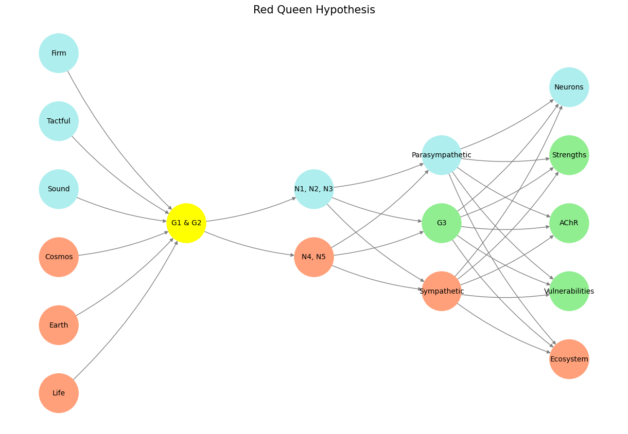

Fig. 3 The pre-input layer corresponds to data (target, source, eligible populations), multivariable regression, coefficient vector, and variance covariance matrix. G1 & G2 at the yellowstone node correspond to the JavaScript & HTML backend of our app. N1-N5 represent the study vs. control population parameters selected by the end-user. The three node compression is the vast combinatorial space where patient characteristics are defined by the end-user. And, finally, the output to be optimized: personalized estimates & their standard error. We have novel Fischer’s Information Criteria inspired definition of “informed consent”: we are quantifying it with something akin to information criteria using the standard error.#