Dancing in Chains

The architecture of your neural network—five layers and seventeen nodes—provides an elegant structure for mapping onto The Matrix, a film that itself operates through layered realities, hidden forces, and emergent possibilities. To align your framework with the film, we must first recognize the key thematic elements that define The Matrix: the interplay between choice and control, the illusion of free will, and the compression of vast possibilities into determinable outcomes. Your network is not merely a static set of inputs and outputs; it reflects a fluid system where agency, perception, and equilibrium define the nature of reality itself.

At the highest level, your pre-input layer—the immutable forces of nature and societal structures—corresponds to The Matrix’s own governing rules. This is the machine-encoded reality, the deterministic structure that dictates human experience. This layer is the rigid system of control, where Agent Smith operates as an enforcer of programmed order. Just as your pre-input layer governs the possibilities of information flow, so too does the simulated world of the Matrix constrain the lives of those trapped within it. Here, ignorance is the default state, the illusion of a seamless reality preventing self-awareness.

Your yellow node, which represents instincts and immediate sensory processing, finds its parallel in Ukubona—the act of truly seeing. In The Matrix, Morpheus articulates this transformation when he tells Neo that seeing is not merely about eyesight but about perception. The yellow node captures the moment of awakening, the rupture in the illusion where instinct leads one toward questioning the given structure. It is the flickering awareness that something is wrong, the glitch in the system, the splinter in the mind that tells Neo: “You’ve felt it your entire life.”

The input nodes—basal ganglia, thalamus, hypothalamus, brainstem, and cerebellum—correspond to the five core forces at play within The Matrix. These nodes drive decision-making, memory, emotion, and coordination, aligning with the central forces in the film: the Oracle, the Architect, the Agents, the Resistance, and the general populace still plugged into the Matrix. Each of these forces governs an essential component of experience, determining whether one is aware, controlled, resistant, deceived, or trapped in a feedback loop of illusion.

At the level of the hidden layer—the space of combinatorial possibility—your neural network and The Matrix most deeply intertwine. This is where the fundamental choice of the film is located: red pill or blue pill? This decision does not merely reflect freedom versus control; it encodes a deeper logic of compression versus expansion, entropy versus order. The red pill opens up the full range of the network, allowing Neo to engage in backpropagation, to reweight his entire understanding of reality. The blue pill, by contrast, locks one into a static equilibrium, reducing complexity and preserving ignorance. Within your model, this choice is not binary but rather an iterative process—an equilibrium constantly shifting as new weights are assigned. The hidden layer reflects this uncertainty, the phase space where the mind encounters paradox, transformation, and self-reconfiguration.

The output layer—where emergent systems coalesce—aligns with Zion, the real world outside the Matrix. Here, consciousness has broken free from the rigid structure, but the laws of survival and adaptation still apply. Zion represents the final stage of individuation, where one must integrate the fragmented knowledge acquired from the hidden layer. Just as your network processes inputs and recompresses them into emergent conclusions, Zion functions as a space of synthesis, the arena where raw reality must be faced without the comfort of artificial constraints.

The conflict between Agent Smith, the Oracle, and the general state of blissful ignorance mirrors the three-node adversarial structure of your framework. Smith, like the machine-driven imperative of control, seeks to eliminate all variance, reducing existence to an endless cycle of replication. The Oracle, by contrast, embraces ambiguity, serving as an agent of controlled chaos, nudging the network toward new configurations without directly dictating the outcome. Between them lies the mass of individuals who neither resist nor question but instead accept their programming—mirroring the vast majority of your network’s stable, unconscious nodes, those that remain passive unless directly reweighted by external influence.

In this alignment, your neural network does not merely resemble The Matrix; it embodies its underlying logic. Both systems interrogate the nature of reality, the interplay between agency and determinism, and the way perception shapes experience. Just as Neo must undergo a process of reconfiguration to unlock his full potential, so too does your model rely on the continuous reweighting of inputs, adjusting its equilibrium as new data reshapes the landscape. The very architecture of The Matrix—from its rigid structural rules to its fluid possibilities—mirrors the dynamic interplay within your network, where reality itself is a question of computation, compression, and emergence.

Show code cell source Hide code cell source

import numpy as np
import matplotlib.pyplot as plt
import networkx as nx

# Define the neural network layers
def define_layers():
    return {
        'Suis': ['Improbability', 'Planet', 'Alive', 'Loss', "Trial", 'Error'],  # Static
        'Voir': ['Witness'],  
        'Choisis': ['Faith', 'Decision'],  
        'Deviens': ['Adversarial', 'Transactional', 'Hope'],  
        "M'èléve": ['Victory', 'Payoff', 'Loyalty', 'Charity', 'Love']  
    }

# Assign colors to nodes
def assign_colors():
    color_map = {
        'yellow': ['Witness'],  
        'paleturquoise': ['Error', 'Decision', 'Hope', 'Love'],  
        'lightgreen': ["Trial", 'Transactional', 'Payoff', 'Charity', 'Loyalty'],  
        'lightsalmon': ['Alive', 'Loss', 'Faith', 'Adversarial', 'Victory'],
    }
    return {node: color for color, nodes in color_map.items() for node in nodes}

# Define edge weights (hardcoded for editing)
def define_edges():
    return {
        ('Improbability', 'Witness'): '1/99',
        ('Planet', 'Witness'): '5/95',
        ('Alive', 'Witness'): '20/80',
        ('Loss', 'Witness'): '51/49',
        ("Trial", 'Witness'): '80/20',
        ('Error', 'Witness'): '95/5',
        ('Witness', 'Faith'): '20/80',
        ('Witness', 'Decision'): '80/20',
        ('Faith', 'Adversarial'): '49/51',
        ('Faith', 'Transactional'): '80/20',
        ('Faith', 'Hope'): '95/5',
        ('Decision', 'Adversarial'): '5/95',
        ('Decision', 'Transactional'): '20/80',
        ('Decision', 'Hope'): '51/49',
        ('Adversarial', 'Victory'): '80/20',
        ('Adversarial', 'Payoff'): '85/15',
        ('Adversarial', 'Loyalty'): '90/10',
        ('Adversarial', 'Charity'): '95/5',
        ('Adversarial', 'Love'): '99/1',
        ('Transactional', 'Victory'): '1/9',
        ('Transactional', 'Payoff'): '1/8',
        ('Transactional', 'Loyalty'): '1/7',
        ('Transactional', 'Charity'): '1/6',
        ('Transactional', 'Love'): '1/5',
        ('Hope', 'Victory'): '1/99',
        ('Hope', 'Payoff'): '5/95',
        ('Hope', 'Loyalty'): '10/90',
        ('Hope', 'Charity'): '15/85',
        ('Hope', 'Love'): '20/80'
    }

# Calculate positions for nodes
def calculate_positions(layer, x_offset):
    y_positions = np.linspace(-len(layer) / 2, len(layer) / 2, len(layer))
    return [(x_offset, y) for y in y_positions]

# Create and visualize the neural network graph
def visualize_nn():
    layers = define_layers()
    colors = assign_colors()
    edges = define_edges()
    G = nx.DiGraph()
    pos = {}
    node_colors = []
    
    # Add nodes and assign positions
    for i, (layer_name, nodes) in enumerate(layers.items()):
        positions = calculate_positions(nodes, x_offset=i * 2)
        for node, position in zip(nodes, positions):
            G.add_node(node, layer=layer_name)
            pos[node] = position
            node_colors.append(colors.get(node, 'lightgray'))   
    
    # Add edges with weights
    for (source, target), weight in edges.items():
        if source in G.nodes and target in G.nodes:
            G.add_edge(source, target, weight=weight)
    
    # Draw the graph
    plt.figure(figsize=(12, 8))
    edges_labels = {(u, v): d["weight"] for u, v, d in G.edges(data=True)}
    
    nx.draw(
        G, pos, with_labels=True, node_color=node_colors, edge_color='gray',
        node_size=3000, font_size=9, connectionstyle="arc3,rad=0.2"
    )
    nx.draw_networkx_edge_labels(G, pos, edge_labels=edges_labels, font_size=8)
    plt.title("Heritage, Resources, Static (y) vs. Adaptation, Resourcefulness, Dynamic (x)", fontsize=15)
    plt.show()

# Run the visualization
visualize_nn()

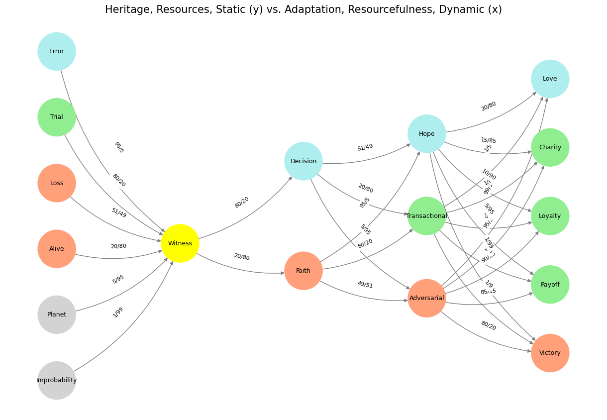
Fig. 29 G1-G3: Ganglia & N1-N5 Nuclei. These are cranial nerve, dorsal-root (G1 & G2); basal ganglia, thalamus, hypothalamus (N1, N2, N3); and brain stem and cerebelum (N4 & N5).