Freedom in Fetters

Fig. 31 The Next Time Your Horse is Behaving Well, Sell it. The numbers in private equity don’t add up because its very much like a betting in a horse race. Too many entrants and exits for anyone to have a reliable dataset with which to estimate odds for any horse-jokey vs. the others for quinella, trifecta, superfecta

Show code cell source Hide code cell source

import numpy as np
import matplotlib.pyplot as plt
import networkx as nx

# Define the neural network layers
def define_layers():
    return {
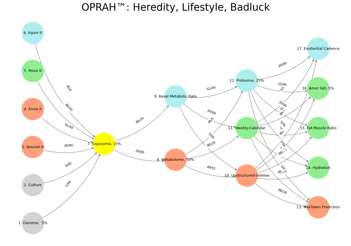
        'Suis': ['Genome,  5%', 'Culture', 'Nourish It', 'Know It', "Move It", 'Injure It'],  # Static
        'Voir': ['Exposome, 15%'],  
        'Choisis': ['Metabolome, 50%', 'Basal Metabolic Rate'],  
        'Deviens': ['Unstructured-Intense', 'Weekly-Calendar', 'Proteome, 25%'],  
        "M'èléve": ['NexToken Prediction', 'Hydration', 'Fat-Muscle Ratio', 'Amor Fatì, 5%', 'Existential Cadence']  
    }

# Assign colors to nodes
def assign_colors():
    color_map = {
        'yellow': ['Exposome, 15%'],  
        'paleturquoise': ['Injure It', 'Basal Metabolic Rate', 'Proteome, 25%', 'Existential Cadence'],  
        'lightgreen': ["Move It", 'Weekly-Calendar', 'Hydration', 'Amor Fatì, 5%', 'Fat-Muscle Ratio'],  
        'lightsalmon': ['Nourish It', 'Know It', 'Metabolome, 50%', 'Unstructured-Intense', 'NexToken Prediction'],
    }
    return {node: color for color, nodes in color_map.items() for node in nodes}

# Define edge weights (hardcoded for editing)
def define_edges():
    return {
        ('Genome,  5%', 'Exposome, 15%'): '1/99',
        ('Culture', 'Exposome, 15%'): '5/95',
        ('Nourish It', 'Exposome, 15%'): '20/80',
        ('Know It', 'Exposome, 15%'): '51/49',
        ("Move It", 'Exposome, 15%'): '80/20',
        ('Injure It', 'Exposome, 15%'): '95/5',
        ('Exposome, 15%', 'Metabolome, 50%'): '20/80',
        ('Exposome, 15%', 'Basal Metabolic Rate'): '80/20',
        ('Metabolome, 50%', 'Unstructured-Intense'): '49/51',
        ('Metabolome, 50%', 'Weekly-Calendar'): '80/20',
        ('Metabolome, 50%', 'Proteome, 25%'): '95/5',
        ('Basal Metabolic Rate', 'Unstructured-Intense'): '5/95',
        ('Basal Metabolic Rate', 'Weekly-Calendar'): '20/80',
        ('Basal Metabolic Rate', 'Proteome, 25%'): '51/49',
        ('Unstructured-Intense', 'NexToken Prediction'): '80/20',
        ('Unstructured-Intense', 'Hydration'): '85/15',
        ('Unstructured-Intense', 'Fat-Muscle Ratio'): '90/10',
        ('Unstructured-Intense', 'Amor Fatì, 5%'): '95/5',
        ('Unstructured-Intense', 'Existential Cadence'): '99/1',
        ('Weekly-Calendar', 'NexToken Prediction'): '1/9',
        ('Weekly-Calendar', 'Hydration'): '1/8',
        ('Weekly-Calendar', 'Fat-Muscle Ratio'): '1/7',
        ('Weekly-Calendar', 'Amor Fatì, 5%'): '1/6',
        ('Weekly-Calendar', 'Existential Cadence'): '1/5',
        ('Proteome, 25%', 'NexToken Prediction'): '1/99',
        ('Proteome, 25%', 'Hydration'): '5/95',
        ('Proteome, 25%', 'Fat-Muscle Ratio'): '10/90',
        ('Proteome, 25%', 'Amor Fatì, 5%'): '15/85',
        ('Proteome, 25%', 'Existential Cadence'): '20/80'
    }

# Calculate positions for nodes
def calculate_positions(layer, x_offset):
    y_positions = np.linspace(-len(layer) / 2, len(layer) / 2, len(layer))
    return [(x_offset, y) for y in y_positions]

# Create and visualize the neural network graph
def visualize_nn():
    layers = define_layers()
    colors = assign_colors()
    edges = define_edges()
    G = nx.DiGraph()
    pos = {}
    node_colors = []
    
    # Create mapping from original node names to numbered labels
    mapping = {}
    counter = 1
    for layer in layers.values():
        for node in layer:
            mapping[node] = f"{counter}. {node}"
            counter += 1
            
    # Add nodes with new numbered labels and assign positions
    for i, (layer_name, nodes) in enumerate(layers.items()):
        positions = calculate_positions(nodes, x_offset=i * 2)
        for node, position in zip(nodes, positions):
            new_node = mapping[node]
            G.add_node(new_node, layer=layer_name)
            pos[new_node] = position
            node_colors.append(colors.get(node, 'lightgray'))
    
    # Add edges with updated node labels
    for (source, target), weight in edges.items():
        if source in mapping and target in mapping:
            new_source = mapping[source]
            new_target = mapping[target]
            G.add_edge(new_source, new_target, weight=weight)
    
    # Draw the graph
    plt.figure(figsize=(12, 8))
    edges_labels = {(u, v): d["weight"] for u, v, d in G.edges(data=True)}
    
    nx.draw(
        G, pos, with_labels=True, node_color=node_colors, edge_color='gray',
        node_size=3000, font_size=9, connectionstyle="arc3,rad=0.2"
    )
    nx.draw_networkx_edge_labels(G, pos, edge_labels=edges_labels, font_size=8)
    plt.title("OPRAH™: Heredity, Lifestyle, Badluck", fontsize=25)
    plt.show()

# Run the visualization
visualize_nn()

Fig. 32 Musical Grammar & Prosody. From a pianist’s perspective, the left hand serves as the foundational architect, voicing the mode and defining the musical landscape—its space and grammar—while the right hand acts as the expressive wanderer, freely extending and altering these modal terrains within temporal pockets, guided by prosody and cadence. In R&B, this interplay often manifests through rich harmonic extensions like 9ths, 11ths, and 13ths, with chromatic passing chords and leading tones adding tension and color. Music’s evocative power lies in its ability to transmit information through a primal, pattern-recognizing architecture, compelling listeners to classify what they hear as either nurturing or threatening—feeding and breeding or fight and flight. This makes music a high-risk, high-reward endeavor, where success hinges on navigating the fine line between coherence and error. Similarly, pattern recognition extends to literature, as seen in Ulysses, where a character misinterprets his companion’s silence as mental composition, reflecting on the instructive pleasures of Shakespearean works used to solve life’s complexities. Both music and literature, then, are deeply rooted in the human impulse to decode and derive meaning, whether through harmonic landscapes or textual introspection. Source: Ulysses, DeepSeek & Yours Truly!