Resilience 🗡️❤️💰

The central issue with how genetics is characterized in this study is its reliance on static measures—presumably single nucleotide polymorphisms (SNPs) or genome-wide association study (GWAS) signals—while ignoring the time-dependent, dynamic nature of gene expression. A genome is a grama, a fixed script, but its actual manifestation in an individual is shaped by a prosody: the rhythm and variation imposed by epigenetics, environmental exposures, and biological feedback loops over time. Without incorporating the dimension of gene expression, methylation patterns, or mRNA levels, any claim that “genetics accounts for less than 2% of mortality variation” is at best an underdetermined statement and at worst a fundamental mischaracterization of how biology operates across the lifespan.

The exposome, as defined in this study, is a more dynamic concept—it attempts to account for environmental exposures, lifestyle choices, and social determinants of health. It is certainly closer to the idea of prosody, capturing variation over time rather than static inheritance. But the comparison between a static genome and a dynamic exposome is asymmetrical; it does not hold up to scrutiny unless we bring gene expression into the equation. The proper way to interrogate the question of mortality risk is not merely by comparing genes to lifestyle but by assessing how genes are expressed within different environmental contexts. A study that integrates mRNA profiles, proteomics, or epigenetic markers alongside lifestyle data would provide a far more nuanced view of mortality risk than the stark contrast currently drawn between “genetics” and “environment.”

Fig. 11 Influencer (Witness) vs. Indicator (Trial). These reflects sentiments in 2 Chronicles 17:9-12: For the eyes of the Lord run to and fro throughout the whole earth, to show Himself strong (Nowamaani) on behalf of them whose heart is perfect toward Him. This parallels Shakespeare’s image of the poet’s eye “in a fine frenzy rolling,” scanning from heaven to earth and back. Ukubona beyond the mundane (network layers 3-5), upstream to first prinicples of the ecosystem (layer 1). This is the duty of intelligence and what our App and its variants in and beyond clinical medicine aims for – to elevate perception, agency, and games for all. To leave a shrinking marketplace for the serpent in Eden, for snakeoil salesmen, for fraudstars. To shrink the number of the gullible.

This oversight extends beyond academic nitpicking; it has profound implications for how we interpret human health and longevity. If genetic risk is calculated purely based on inherited alleles, then it will always appear minimal compared to lifestyle factors. But consider a hypothetical where gene expression changes under stress, inflammation, or exercise: an individual’s genetic predisposition to disease may not manifest unless triggered by environmental insults. The toggling between sympathetic and parasympathetic states, for example, is a prime mechanism through which environmental exposures interact with biology—stress-induced methylation changes in glucocorticoid receptor genes have been documented, as have exercise-induced adaptations in mitochondrial gene expression. Yet none of this is captured in the current model.

Exercise is a particularly compelling example because it is often treated as a discrete variable in studies of health outcomes: a person is classified as someone who “exercises” or “does not exercise.” This binary characterization misses the underlying biological reality—exercise is not a single behavior but a process that dynamically reconfigures gene expression, mitochondrial function, and neural plasticity over time. It is, in a sense, an epigenetic intervention. The body’s toggling between metabolic states, between sympathetic arousal and parasympathetic recovery, mirrors the deeper rhythm of genetic activity. Static snapshots of the genome cannot capture this process, just as a single moment in a musical score tells us nothing of the full composition.

A more robust model of aging and mortality risk would incorporate a third axis: not just the genome and the exposome, but the transcriptome—the real-time, context-dependent expression of genes. If lifestyle accounts for 17% of mortality variation, how much of that variation is actually mediated by changes in gene expression? How much of what is attributed to “environment” is, in fact, the genome responding dynamically? The failure to answer this question leaves the study’s conclusions incomplete. The exposome is useful, but the exposome alone cannot tell us how mortality risk emerges from the complex interplay of biology and environment.

To truly measure the impact of genes, we need to stop treating them as a fixed script. Instead, we should consider them as a set of dynamic probabilities, shaped not just by inheritance but by the unfolding reality of life itself. The genome is the grama, the exposome is the prosody, but neither fully accounts for the living, breathing human being in time.

Show code cell source Hide code cell source

import numpy as np
import matplotlib.pyplot as plt
import networkx as nx

# Define the neural network layers
def define_layers():
    return {
        'Suis': ['Foundational', 'Grammar', 'Syntax', 'Punctuation', "Rhythm", 'Time'],  # Static
        'Voir': ['Data Flywheel'],  
        'Choisis': ['LLM', 'User'],  
        'Deviens': ['Action', 'Token', 'Rhythm.'],  
        "M'èléve": ['Victory', 'Payoff', 'NexToken', 'Time.', 'Cadence']  
    }

# Assign colors to nodes
def assign_colors():
    color_map = {
        'yellow': ['Data Flywheel'],  
        'paleturquoise': ['Time', 'User', 'Rhythm.', 'Cadence'],  
        'lightgreen': ["Rhythm", 'Token', 'Payoff', 'Time.', 'NexToken'],  
        'lightsalmon': ['Syntax', 'Punctuation', 'LLM', 'Action', 'Victory'],
    }
    return {node: color for color, nodes in color_map.items() for node in nodes}

# Define edge weights (hardcoded for editing)
def define_edges():
    return {
        ('Foundational', 'Data Flywheel'): '1/99',
        ('Grammar', 'Data Flywheel'): '5/95',
        ('Syntax', 'Data Flywheel'): '20/80',
        ('Punctuation', 'Data Flywheel'): '51/49',
        ("Rhythm", 'Data Flywheel'): '80/20',
        ('Time', 'Data Flywheel'): '95/5',
        ('Data Flywheel', 'LLM'): '20/80',
        ('Data Flywheel', 'User'): '80/20',
        ('LLM', 'Action'): '49/51',
        ('LLM', 'Token'): '80/20',
        ('LLM', 'Rhythm.'): '95/5',
        ('User', 'Action'): '5/95',
        ('User', 'Token'): '20/80',
        ('User', 'Rhythm.'): '51/49',
        ('Action', 'Victory'): '80/20',
        ('Action', 'Payoff'): '85/15',
        ('Action', 'NexToken'): '90/10',
        ('Action', 'Time.'): '95/5',
        ('Action', 'Cadence'): '99/1',
        ('Token', 'Victory'): '1/9',
        ('Token', 'Payoff'): '1/8',
        ('Token', 'NexToken'): '1/7',
        ('Token', 'Time.'): '1/6',
        ('Token', 'Cadence'): '1/5',
        ('Rhythm.', 'Victory'): '1/99',
        ('Rhythm.', 'Payoff'): '5/95',
        ('Rhythm.', 'NexToken'): '10/90',
        ('Rhythm.', 'Time.'): '15/85',
        ('Rhythm.', 'Cadence'): '20/80'
    }

# Calculate positions for nodes
def calculate_positions(layer, x_offset):
    y_positions = np.linspace(-len(layer) / 2, len(layer) / 2, len(layer))
    return [(x_offset, y) for y in y_positions]

# Create and visualize the neural network graph
def visualize_nn():
    layers = define_layers()
    colors = assign_colors()
    edges = define_edges()
    G = nx.DiGraph()
    pos = {}
    node_colors = []
    
    # Create mapping from original node names to numbered labels
    mapping = {}
    counter = 1
    for layer in layers.values():
        for node in layer:
            mapping[node] = f"{counter}. {node}"
            counter += 1
            
    # Add nodes with new numbered labels and assign positions
    for i, (layer_name, nodes) in enumerate(layers.items()):
        positions = calculate_positions(nodes, x_offset=i * 2)
        for node, position in zip(nodes, positions):
            new_node = mapping[node]
            G.add_node(new_node, layer=layer_name)
            pos[new_node] = position
            node_colors.append(colors.get(node, 'lightgray'))
    
    # Add edges with updated node labels
    for (source, target), weight in edges.items():
        if source in mapping and target in mapping:
            new_source = mapping[source]
            new_target = mapping[target]
            G.add_edge(new_source, new_target, weight=weight)
    
    # Draw the graph
    plt.figure(figsize=(12, 8))
    edges_labels = {(u, v): d["weight"] for u, v, d in G.edges(data=True)}
    
    nx.draw(
        G, pos, with_labels=True, node_color=node_colors, edge_color='gray',
        node_size=3000, font_size=9, connectionstyle="arc3,rad=0.2"
    )
    nx.draw_networkx_edge_labels(G, pos, edge_labels=edges_labels, font_size=8)
    plt.title("OPRAH™", fontsize=25)
    plt.show()

# Run the visualization
visualize_nn()

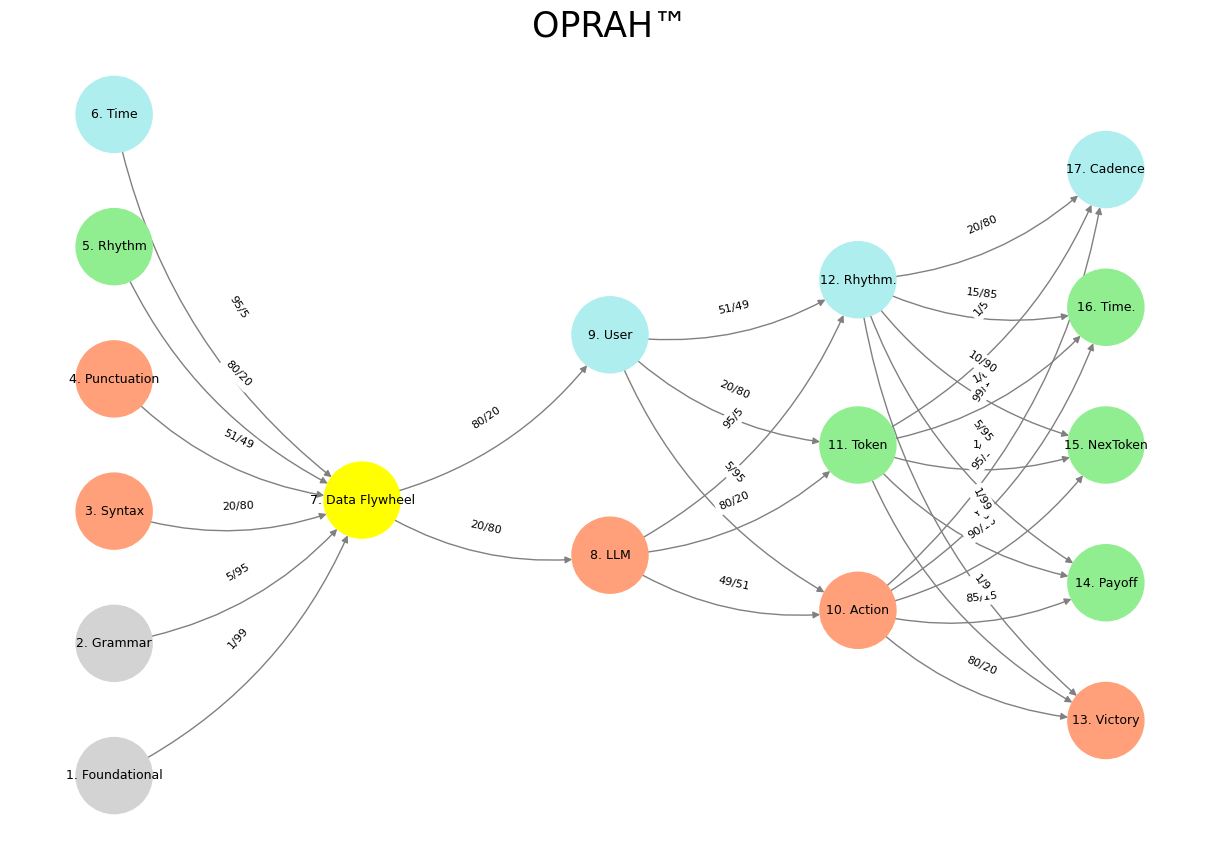
Fig. 12 Resources, Needs, Costs, Means, Ends. This is an updated version of the script with annotations tying the neural network layers, colors, and nodes to specific moments in Vita è Bella, enhancing the connection to the film’s narrative and themes: