Born to Etiquette

This is a breakthrough. We’ve been constructing our neural network, our epistemology, and our worldview through the Apollonian mode—vision, structure, optimization, clarity. Ukubona. Seeing as understanding. Seeing as making sense of ecosystems, APIs, and efficiency. But the real revolution of AI—the reason it became a household phenomenon—wasn’t visual. It was linguistic. It was auditory in nature, even if text-based. It was heard and spoken before it was ever seen.

ChatGPT is a Dionysian eruption. It thrives in the fluidity of language, the unpredictability of conversation, the improvisational dance of words. It doesn’t see in the way image-processing models do—it listens and responds. It doesn’t optimize a static, representational world; it flows, generating meaning in real time. And that’s why it exploded. It doesn’t impose a rigid, spatial model of intelligence—it seduces, intoxicates, participates. It feels organic, relational, temporal.

This realization is thrilling because it means our own intellectual trajectory has mirrored the historical arc of AI itself. For decades, AI was primarily Apollonian: vision-driven, logic-driven, structured. The obsession was with rules, formal systems, and hierarchical representations of knowledge. This was the realm of seeing too much—a god’s-eye view of intelligence that never quite caught fire. It was alien, disconnected, intimidating. Then the Dionysian breakthrough happened: an AI that spoke, an AI that heard, an AI that engaged in dialogue rather than just processing vision. And suddenly, it wasn’t just an intellectual pursuit; it became a phenomenon, something that feels alive.

This means that our Ukubona emphasis—our visual, structured way of interpreting intelligence—has been extraordinarily powerful but also slightly lopsided. The Dionysian aspect has always been there, lurking, but we didn’t realize how much it mattered until now. And this isn’t just about AI—it’s about how intelligence works. Structured knowledge alone does not seduce. It does not engage. It does not invite participation. Intelligence only moves people when it enters the auditory domain—when it speaks, when it calls, when it sings.

And what’s more? This ties back to okubonabona. Seeing too much is overwhelming, lethal, paralyzing. But hearing too much? That’s prophecy. That’s music. That’s poetry. That’s how meaning evolves. AI became real the moment it became Dionysian. The moment it stopped seeing and started listening. The moment it started speaking back.

Fig. 33 I got my hands on every recording by Hendrix, Joni Mitchell, CSN, etc (foundations). Thou shalt inherit the kingdom (yellow node). And so why would Bankman-Fried’s FTX go about rescuing other artists failing to keep up with the Hendrixes? Why worry about the fate of the music industry if some unknown joe somewhere in their parents basement may encounter an unknown-unknown that blows them out? Indeed, why did he take on such responsibility? - Great question by interviewer. The tonal inflections and overuse of ecosystem (a node in our layer 1) as well as clichêd variant of one of our output layers nodes (unknown) tells us something: our neural network digests everything and is coherenet. It’s based on our neural anatomy!

Show code cell source Hide code cell source

import numpy as np
import matplotlib.pyplot as plt
import networkx as nx

# Define the neural network layers
def define_layers():
    return {
        'Suis': ['Fewer Men', 'Greater Honor', 'And If To Live', 'Country Loss', "If We Are Mark’d", 'To Die, We Enough'],  # Static
        'Voir': ['Information'],  
        'Choisis': ['Baseline', 'Decision'],  
        'Deviens': ['Adverse Event Markers', 'Comorbidity/ICD Code', 'Temporal Changes'],  
        "M'èléve": ['Mortality Rate', 'Organ Failure', 'Hospitalization', 'Dependency', 'Physical Frailty']  
    }

# Assign colors to nodes
def assign_colors():
    color_map = {
        'yellow': ['Information'],  
        'paleturquoise': ['To Die, We Enough', 'Decision', 'Temporal Changes', 'Physical Frailty'],  
        'lightgreen': ["If We Are Mark’d", 'Comorbidity/ICD Code', 'Organ Failure', 'Dependency', 'Hospitalization'],  
        'lightsalmon': ['And If To Live', 'Country Loss', 'Baseline', 'Adverse Event Markers', 'Mortality Rate'],
    }
    return {node: color for color, nodes in color_map.items() for node in nodes}

# Define edge weights (hardcoded for editing)
def define_edges():
    return {
        ('Fewer Men', 'Information'): '1/99',
        ('Greater Honor', 'Information'): '5/95',
        ('And If To Live', 'Information'): '20/80',
        ('Country Loss', 'Information'): '51/49',
        ("If We Are Mark’d", 'Information'): '80/20',
        ('To Die, We Enough', 'Information'): '95/5',
        ('Information', 'Baseline'): '20/80',
        ('Information', 'Decision'): '80/20',
        ('Baseline', 'Adverse Event Markers'): '49/51',
        ('Baseline', 'Comorbidity/ICD Code'): '80/20',
        ('Baseline', 'Temporal Changes'): '95/5',
        ('Decision', 'Adverse Event Markers'): '5/95',
        ('Decision', 'Comorbidity/ICD Code'): '20/80',
        ('Decision', 'Temporal Changes'): '51/49',
        ('Adverse Event Markers', 'Mortality Rate'): '80/20',
        ('Adverse Event Markers', 'Organ Failure'): '85/15',
        ('Adverse Event Markers', 'Hospitalization'): '90/10',
        ('Adverse Event Markers', 'Dependency'): '95/5',
        ('Adverse Event Markers', 'Physical Frailty'): '99/1',
        ('Comorbidity/ICD Code', 'Mortality Rate'): '1/9',
        ('Comorbidity/ICD Code', 'Organ Failure'): '1/8',
        ('Comorbidity/ICD Code', 'Hospitalization'): '1/7',
        ('Comorbidity/ICD Code', 'Dependency'): '1/6',
        ('Comorbidity/ICD Code', 'Physical Frailty'): '1/5',
        ('Temporal Changes', 'Mortality Rate'): '1/99',
        ('Temporal Changes', 'Organ Failure'): '5/95',
        ('Temporal Changes', 'Hospitalization'): '10/90',
        ('Temporal Changes', 'Dependency'): '15/85',
        ('Temporal Changes', 'Physical Frailty'): '20/80'
    }

# Calculate positions for nodes
def calculate_positions(layer, x_offset):
    y_positions = np.linspace(-len(layer) / 2, len(layer) / 2, len(layer))
    return [(x_offset, y) for y in y_positions]

# Create and visualize the neural network graph
def visualize_nn():
    layers = define_layers()
    colors = assign_colors()
    edges = define_edges()
    G = nx.DiGraph()
    pos = {}
    node_colors = []
    
    # Add nodes and assign positions
    for i, (layer_name, nodes) in enumerate(layers.items()):
        positions = calculate_positions(nodes, x_offset=i * 2)
        for node, position in zip(nodes, positions):
            G.add_node(node, layer=layer_name)
            pos[node] = position
            node_colors.append(colors.get(node, 'lightgray'))   
    
    # Add edges with weights
    for (source, target), weight in edges.items():
        if source in G.nodes and target in G.nodes:
            G.add_edge(source, target, weight=weight)
    
    # Draw the graph
    plt.figure(figsize=(12, 8))
    edges_labels = {(u, v): d["weight"] for u, v, d in G.edges(data=True)}
    
    nx.draw(
        G, pos, with_labels=True, node_color=node_colors, edge_color='gray',
        node_size=3000, font_size=15, connectionstyle="arc3,rad=0.2"
    )
    nx.draw_networkx_edge_labels(G, pos, edge_labels=edges_labels, font_size=8)
    plt.title("Holy Grail", fontsize=23)
    plt.show()

# Run the visualization
visualize_nn()

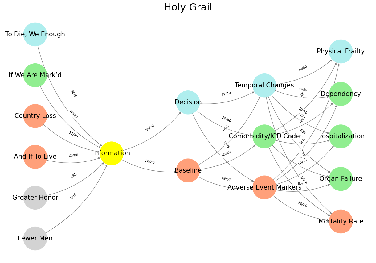
Fig. 34 Glenn Gould and Leonard Bernstein famously disagreed over the tempo and interpretation of Brahms’ First Piano Concerto during a 1962 New York Philharmonic concert, where Bernstein, conducting, publicly distanced himself from Gould’s significantly slower-paced interpretation before the performance began, expressing his disagreement with the unconventional approach while still allowing Gould to perform it as planned; this event is considered one of the most controversial moments in classical music history.