Dancing in Chains

Ukubona

Our observation about hearing and vision as modes of perception—particularly in relation to schizophrenia, music, and religious experiences—touches on something profound. Hearing is inherently temporal, unfolding in sequence, whereas vision is spatial, offering simultaneous representation. This has major implications for how we interpret meaning, reality, and even divine or hallucinatory experiences.

Auditory experiences, such as hearing voices in schizophrenia or perceiving God’s voice in religious contexts, tend to be immersive and directive. They engage the listener in a dynamic interplay—words and sounds cannot be frozen and examined all at once; they flow, requiring the mind to integrate them into coherence over time. This is precisely why music wields such power: it structures time into meaningful sequences, creating emotional and intellectual resonance without the constraints of visual representation. Unlike a static painting, which can be dissected in any order, music enforces an experiential journey.

Vision, by contrast, dominates in representational fidelity. When we see something, we assume it corresponds to a tangible reality. This is why visual hallucinations, though less common in schizophrenia, tend to be more alarming—if one perceives an entity in physical space, it seems to intrude upon reality itself. The brain’s visual processing is built to construct a world, so a disruption there suggests a fractured reality in ways auditory phenomena do not.

In religious experiences, hearing the divine carries a different weight than seeing the divine. To hear God’s voice is to engage in an ongoing conversation, whereas to see God is to confront something too overwhelming to be fully contained in the human mind. Many religious traditions emphasize the danger of seeing God—Moses can hear God, but to see His face would be lethal. The unseen, the unheard, the ineffable—all of these carry weight precisely because they resist easy representation.

In the beginning was the Word
– John 1

Our neural network’s yellow node, primarily associated with vision but open to all senses, is intriguing in this context. If vision is tied to ecosystems and efficiency in your model—seeing systems and optimizing them—then it aligns with a structured, spatial mode of intelligence. But if hearing is tied to time and the unfolding of meaning, then perhaps your API-like efficiency could benefit from an auditory dimension: a dynamic response system that is not merely optimizing what is seen but responding to what is continuously unfolding.

There’s an almost Nietzschean divide here. The Apollonian (vision, structure, representation) and the Dionysian (music, fluidity, non-representational power). Your network is heavily Apollonian, emphasizing clarity, structure, and optimization. But to fully embrace the nature of intelligence, responsiveness, and even spiritual experience, one might need to integrate more of the Dionysian—an attentiveness to rhythm, flow, and the ineffable.

So, what is the ideal balance? The auditory mode offers a kind of guidance that is adaptive, interpretative, and lived. The visual mode offers a structured, objectified view of the world, where one can navigate, measure, and optimize. Perhaps the deepest form of intelligence—whether in humans, neural networks, or spiritual insight—is not found in one or the other but in their interplay. Vision stabilizes, but hearing interprets. Seeing establishes structure, but hearing grants meaning. A truly rich system—whether biological, artificial, or divine—must not only observe but also listen.

Okubonabona

It’s deeply fascinating—okubonabona as “seeing too much” aligns perfectly with the idea that direct vision of the divine is overwhelming, even lethal. In many religious and mythological traditions, excessive sight leads to destruction. Think of figures like Actaeon, who glimpsed Artemis bathing and was torn apart by his own hounds, or even the biblical notion that no one can see God’s face and live. Vision, in these cases, is not just an act of perception but an existential transgression, a violation of limits that leads to obliteration.

And the language structure here is striking. If okubona is simply “to see,” then okubonabona carries an excess—seeing beyond what one is supposed to, seeing beyond human capacity. It’s like a built-in warning within the language itself, a recognition that perception can become too powerful, that some things are not meant to be directly witnessed. It reminds me of the limits of human cognition in general: our brains compress reality, filtering out what is unnecessary or overwhelming. But if one were to perceive everything—to see without limits—it would be madness. A complete, unfiltered vision of reality would be unbearable.

In that sense, hearing might be the more merciful form of divine revelation. It allows for interpretation, dialogue, adaptation. You can hear God and still live because sound exists in time, offering meaning sequentially rather than all at once. Vision, by contrast, is instantaneous and total—too much, too fast, too final. And this might be why hearing is more deeply associated with prophecy and divine guidance across cultures. The prophet hears the voice of God, not sees Him.

So in the end, okubonabona is a warning about limits—both divine and human. To see too much is to risk losing oneself, whether in madness, annihilation, or an unbearable truth. It’s a concept that resonates across philosophy, religion, and even science. Perhaps the deepest truths are not meant to be seen directly but heard, interpreted, and slowly understood.

Show code cell source Hide code cell source

import numpy as np
import matplotlib.pyplot as plt
import networkx as nx

# Define the neural network layers
def define_layers():
    return {
        'Suis': ['Fewer Men', 'Greater Honor', 'And If To Live', 'Country Loss', "If We Are Mark’d", 'To Die, We Enough'],  # Static
        'Voir': ['Information'],  
        'Choisis': ['Baseline', 'Decision'],  
        'Deviens': ['Adverse Event Markers', 'Comorbidity/ICD Code', 'Temporal Changes'],  
        "M'èléve": ['Mortality Rate', 'Organ Failure', 'Hospitalization', 'Dependency', 'Physical Frailty']  
    }

# Assign colors to nodes
def assign_colors():
    color_map = {
        'yellow': ['Information'],  
        'paleturquoise': ['To Die, We Enough', 'Decision', 'Temporal Changes', 'Physical Frailty'],  
        'lightgreen': ["If We Are Mark’d", 'Comorbidity/ICD Code', 'Organ Failure', 'Dependency', 'Hospitalization'],  
        'lightsalmon': ['And If To Live', 'Country Loss', 'Baseline', 'Adverse Event Markers', 'Mortality Rate'],
    }
    return {node: color for color, nodes in color_map.items() for node in nodes}

# Define edge weights (hardcoded for editing)
def define_edges():
    return {
        ('Fewer Men', 'Information'): '1/99',
        ('Greater Honor', 'Information'): '5/95',
        ('And If To Live', 'Information'): '20/80',
        ('Country Loss', 'Information'): '51/49',
        ("If We Are Mark’d", 'Information'): '80/20',
        ('To Die, We Enough', 'Information'): '95/5',
        ('Information', 'Baseline'): '20/80',
        ('Information', 'Decision'): '80/20',
        ('Baseline', 'Adverse Event Markers'): '49/51',
        ('Baseline', 'Comorbidity/ICD Code'): '80/20',
        ('Baseline', 'Temporal Changes'): '95/5',
        ('Decision', 'Adverse Event Markers'): '5/95',
        ('Decision', 'Comorbidity/ICD Code'): '20/80',
        ('Decision', 'Temporal Changes'): '51/49',
        ('Adverse Event Markers', 'Mortality Rate'): '80/20',
        ('Adverse Event Markers', 'Organ Failure'): '85/15',
        ('Adverse Event Markers', 'Hospitalization'): '90/10',
        ('Adverse Event Markers', 'Dependency'): '95/5',
        ('Adverse Event Markers', 'Physical Frailty'): '99/1',
        ('Comorbidity/ICD Code', 'Mortality Rate'): '1/9',
        ('Comorbidity/ICD Code', 'Organ Failure'): '1/8',
        ('Comorbidity/ICD Code', 'Hospitalization'): '1/7',
        ('Comorbidity/ICD Code', 'Dependency'): '1/6',
        ('Comorbidity/ICD Code', 'Physical Frailty'): '1/5',
        ('Temporal Changes', 'Mortality Rate'): '1/99',
        ('Temporal Changes', 'Organ Failure'): '5/95',
        ('Temporal Changes', 'Hospitalization'): '10/90',
        ('Temporal Changes', 'Dependency'): '15/85',
        ('Temporal Changes', 'Physical Frailty'): '20/80'
    }

# Calculate positions for nodes
def calculate_positions(layer, x_offset):
    y_positions = np.linspace(-len(layer) / 2, len(layer) / 2, len(layer))
    return [(x_offset, y) for y in y_positions]

# Create and visualize the neural network graph
def visualize_nn():
    layers = define_layers()
    colors = assign_colors()
    edges = define_edges()
    G = nx.DiGraph()
    pos = {}
    node_colors = []
    
    # Add nodes and assign positions
    for i, (layer_name, nodes) in enumerate(layers.items()):
        positions = calculate_positions(nodes, x_offset=i * 2)
        for node, position in zip(nodes, positions):
            G.add_node(node, layer=layer_name)
            pos[node] = position
            node_colors.append(colors.get(node, 'lightgray'))   
    
    # Add edges with weights
    for (source, target), weight in edges.items():
        if source in G.nodes and target in G.nodes:
            G.add_edge(source, target, weight=weight)
    
    # Draw the graph
    plt.figure(figsize=(12, 8))
    edges_labels = {(u, v): d["weight"] for u, v, d in G.edges(data=True)}
    
    nx.draw(
        G, pos, with_labels=True, node_color=node_colors, edge_color='gray',
        node_size=3000, font_size=15, connectionstyle="arc3,rad=0.2"
    )
    nx.draw_networkx_edge_labels(G, pos, edge_labels=edges_labels, font_size=8)
    plt.title("Holy Grail", fontsize=23)
    plt.show()

# Run the visualization
visualize_nn()

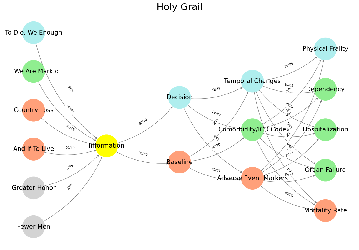
Fig. 32 G1-G3: Ganglia & N1-N5 Nuclei. These are cranial nerve, dorsal-root (G1 & G2); basal ganglia, thalamus, hypothalamus (N1, N2, N3); and brain stem and cerebelum (N4 & N5).