1

Show code cell source Hide code cell source

suppressWarnings({
  invisible({
    rm(list = ls())

    if (!require(icdpicr, quietly = TRUE, warn.conflicts = FALSE)) install.packages('icdpicr')
    if (!require(dplyr, quietly = TRUE, warn.conflicts = FALSE)) install.packages('dplyr')
    if (!require(readr, quietly = TRUE, warn.conflicts = FALSE)) install.packages('readr')
    if (!require(tidyr, quietly = TRUE, warn.conflicts = FALSE)) install.packages('tidyr')
    if (!require(ggplot2, quietly = TRUE, warn.conflicts = FALSE)) install.packages('ggplot2')
    if (!require(gganimate, quietly = TRUE, warn.conflicts = FALSE)) install.packages('gganimate')
    if (!require(magick, quietly = TRUE, warn.conflicts = FALSE)) install.packages('magick')
    if (!require(gifski, quietly = TRUE, warn.conflicts = FALSE)) install.packages('gifski')

    library(icdpicr, quietly = TRUE, warn.conflicts = FALSE)
    library(dplyr, quietly = TRUE, warn.conflicts = FALSE)
    library(readr, quietly = TRUE, warn.conflicts = FALSE)
    library(tidyr, quietly = TRUE, warn.conflicts = FALSE)
    library(ggplot2, quietly = TRUE, warn.conflicts = FALSE)
    library(gganimate, quietly = TRUE, warn.conflicts = FALSE)
    library(magick, quietly = TRUE, warn.conflicts = FALSE)
    library(gifski, quietly = TRUE, warn.conflicts = FALSE)
  })
})

The downloaded binary packages are in
	/var/folders/sx/fd6zgj191mx45hspzbgwzlnr0000gn/T//RtmpuceRvB/downloaded_packages

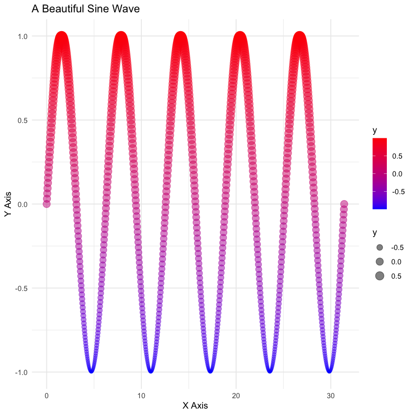
2

Show code cell source Hide code cell source

# Loading required libraries
library(ggplot2)

# Creating a data frame with 1,000 points following a sine wave
n_points <- 1000
data <- data.frame(
  x = seq(0, 10 * pi, length.out = n_points),
  y = sin(seq(0, 10 * pi, length.out = n_points))
)

# Using ggplot2 to create the plot
ggplot(data, aes(x = x, y = y, color = y, size = y)) +
  geom_point(alpha = 0.5) +
  scale_color_gradient(low = "blue", high = "red") +
  scale_size_continuous(range = c(1, 5)) +
  theme_minimal() +
  labs(title = "A Beautiful Sine Wave",
       x = "X Axis",
       y = "Y Axis")

3

Show code cell source Hide code cell source

fibonacci <- local({
  memo <- numeric()
  function(n) {
    if (n <= 1) return(n)
    if (!is.na(memo[n])) return(memo[n])
    memo[n] <<- fibonacci(n - 1) + fibonacci(n - 2)
    return(memo[n])
  }
})

# Example usage
n <- 10
cat("The first", n, "numbers in the Fibonacci sequence are:")
sapply(0:(n-1), fibonacci)

The first 10 numbers in the Fibonacci sequence are:

1. 0
2. 1
3. 1
4. 2
5. 3
6. 5
7. 8
8. 13
9. 21
10. 34

4

Show code cell source Hide code cell source

# Loading libraries
library(ggplot2)
library(gganimate)

# Defining parameters for a particle in a magnetic field
t <- seq(0, 10, by = 0.1)
x <- sin(t)
y <- cos(t)

# Creating a data frame to hold the values
particle_data <- data.frame(
  time = t,
  x = x,
  y = y
)

# Creating the plot using ggplot2 and gganimate
plot <- ggplot(particle_data, aes(x = x, y = y)) +
  geom_path(aes(group = 1), color = 'gray') + # Making sure all points are in the same group
  geom_point(size = 4) +
  labs(title = "Particle in a Magnetic Field",
       x = "X Axis",
       y = "Y Axis") +
  theme_minimal() +
  coord_fixed(ratio = 1) +
  transition_reveal(time)

# Create and save the animation
animate(plot, renderer = gifski_renderer("particle_animation.gif"))

`geom_path()`: Each group consists of only one observation.
i Do you need to adjust the group aesthetic?
`geom_path()`: Each group consists of only one observation.
i Do you need to adjust the group aesthetic?