Show code cell source Hide code cell source

import matplotlib.pyplot as plt
import numpy as np

# Create data for the skill and challenge levels
skill_levels = np.linspace(0, 10, 100)
challenge_levels = np.linspace(0, 10, 100)

# Define the flow channel boundaries
flow_channel = skill_levels

# Adjust the phase and amplitude of the sinusoid wave
phase = np.pi / 16  # Reducing the wavelength by a quarter
amplitude = 1.5
flow_channel += np.sin(skill_levels + phase) * amplitude

# Define the yellow zone boundaries
yellow_zone_low = flow_channel - 1.5
yellow_zone_high = flow_channel + 1.5

# Define the sinusoid function with the middle yellow line as its axis
sinusoid = flow_channel + np.sin(skill_levels + phase) * amplitude

# Define the anxiety and boredom areas
anxiety_area = np.where(challenge_levels > flow_channel, challenge_levels, np.nan)
boredom_area = np.where(challenge_levels < flow_channel, challenge_levels, np.nan)

# Plotting
plt.figure(figsize=(8, 6))

# Plot the anxiety and boredom areas
plt.fill_between(skill_levels, flow_channel, 10, color='red', alpha=0.3, label='Place/Identification', interpolate=True)
plt.fill_between(skill_levels, 0, flow_channel, color='green', alpha=0.3, label='Time/Revelation', interpolate=True)
plt.fill_between(skill_levels, yellow_zone_low, yellow_zone_high, color='yellow', alpha=0.3, label='Agent/Evolution', interpolate=True)

# Plot the sinusoid function
plt.plot(skill_levels, sinusoid, color='purple', linestyle='-')

# Add arrowhead to the sinusoid line (flipped direction)
plt.arrow(skill_levels[-2], sinusoid[-2], skill_levels[-1] - skill_levels[-2], sinusoid[-1] - sinusoid[-2],
          color='purple', length_includes_head=True, head_width=-0.15, head_length=-0.3)

# Plot the flow channel boundaries
plt.plot(skill_levels, flow_channel, color='yellow', linestyle='-')

# Set plot labels and title
plt.xlabel('skill-level')
plt.ylabel('challenge-level', rotation='horizontal', ha='right')  # Rotate the label horizontally

# Set plot limits and grid
plt.xlim(0, 10)
plt.ylim(0, 10)
plt.grid(True)

# Set tick labels
tick_labels = ['0', '2', '4', '6', '8', '10']
plt.xticks(np.linspace(0, 10, 6), tick_labels)
plt.yticks(np.linspace(0, 10, 6), tick_labels)

# Add text annotations to label the areas
plt.text(1, 6, 'anxiety', color='black', ha='center', va='center', fontsize=12, bbox=dict(facecolor='pink', edgecolor='pink', boxstyle='round'))
plt.text(4.5, 4.5, 'flow', color='black', ha='center', va='center', fontsize=12, bbox=dict(facecolor='yellow', edgecolor='yellow', boxstyle='round'))
plt.text(8, 3, 'boredom', color='black', ha='center', va='center', fontsize=12, bbox=dict(facecolor='lightgreen', edgecolor='lightgreen', boxstyle='round'))

# Display the plot
plt.show()

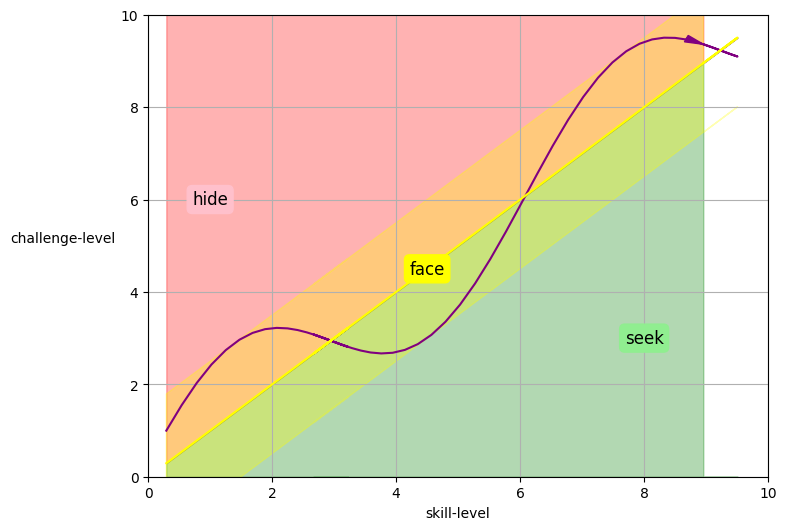
1. face the unending chain of worthy adversaries lined up for us

2. seek out he that was, is, ever shall be pinacle of hierarchy

3. hide in silos of our own making, with kindred spirits