Stata

Stata I (Basic)

• Commands, syntax, and file management restricted to Stata dropdown menu, command window, and .do files on local computer

Stata II (Intermediate)

• File management including .do, .ado, and datafiles are managed remotely on GitHub to enhance collaboration, sharing, and openness

Stata III (Advanced)

• Batch mode is used on a Visual Studio Code terminal with .sh scripts, with .do files and other outputs embedded in .ipynb env. Alternatively, .ipynb codeblocks are used with a Stata kernel, in the same way as is done while running R with an R kernel. This completely mimics the Python environment and Stata and R applications needn’t ever be opened. RMarkdown has absolutely no advanced over a Jupyter book.

Victory! But After 100 Iterations!!

Just scored a victory that carries profound implications for “Stata III (Advanced)”

It looks like the Stata kernel (stata) is listed as an available kernel, which is a good sign. Since you’re still not seeing it in the kernel selector in VS Code, it might be worth checking the VS Code settings to ensure it’s looking in the correct directory for kernels.

In VS Code, you can check the Jupyter kernel settings by going to the command palette (Ctrl+Shift+P) and searching for “Preferences: Open Settings (UI)”. Then, navigate to the “Python > Jupyter” section and look for the “Jupyter: Kernel Spec Path” setting. Make sure it’s pointing to the correct directory where the Stata kernel is installed (/Users/d/Library/Jupyter/kernels/ in your case).

If the path is correct and you’re still not seeing the Stata kernel, you might try restarting VS Code again or even restarting your computer to see if that resolves the issue. Sometimes, these changes require a complete restart to take effect.

# Workflow for Stata III 
export PATH=$PATH:/applications/stata/statamp.app/contents/macos/
stata-mp -b work/abikesa_batch.do

Ah, I see what you’re trying to do. Running Stata in batch mode is a handy way to automate tasks, especially when dealing with large datasets or repetitive tasks.

To run a remote script in batch mode with Stata, you can use the curl command to download the script from GitHub and then pass it to Stata for execution. Here’s how you can do it:

# Download the remote script using curl
curl -O https://github.com/abikesa/do/raw/main/hello.do

# Run Stata in batch mode with the downloaded script
export PATH=$PATH:/applications/stata/statamp.app/contents/macos/
stata-mp -b hello.do

This script will download the hello.do script from the GitHub repository and then execute it in batch mode using Stata. Make sure you have curl installed on your system, or you can use any other tool to download files from the web.

Running scripts remotely can be a powerful tool, but always ensure you trust the source of the script to avoid any security risks.

display "Hello, Stata!"

Hello, Stata!

Nonparametric

Show code cell source Hide code cell source

qui {
capture log close 
log using jamascript.log, replace 
global repo https://github.com/muzaale/forum/raw/main/ 
// cls; some commands don't work outside Stata!!
/*noi di "What is your work directory?" _request(workdir)
if "$workdir" == "" {
	di as err "Please provide your work directory"
	exit
}
else {
	cd $workdir
	noi di "jamascript is running ..."
}
*/
use ${repo}esrdRisk_t02tT, clear
tab donor rSMGJcEdF_d
g entry = rSMGJcEdF_t0
//linkage for donors after 2011 is untrustworthy
replace rSMGJcEdF_d=0 if rSMGJcEdF_tT > d(31dec2011)
replace rSMGJcEdF_tT = d(31dec2011) if rSMGJcEdF_tT > d(31dec2011)
//linkage before 1994 is untrustworthy
#delimit ;
replace entry = d(01jan1994) if  
    entry < d(01jan1994) &  
	rSMGJcEdF_tT > d(01jan1994); 
stset rSMGJcEdF_tT,  
    origin(rSMGJcEdF_t0)  
	entry(`entry')  
	fail(rSMGJcEdF_d==2)  
	scale(365.25); 
#delimit cr 
sts list, fail by(donor) at(5 12 15) saving(km, replace ) 
preserve  
    use km, clear  
	replace failure=failure*100
    sum failure if donor==1 & time==5
	local don5y: di %3.2f r(mean)
    sum failure if donor==1 & time==12
	local don12y: di %3.2f r(mean)
	sum failure if donor==1 & time==15
	local don15y: di %3.2f r(mean)
	//
    sum failure if donor==2 & time==5
	local hnd5y: di %3.2f r(mean)
    sum failure if donor==2 & time==12
	local hnd12y: di %3.2f r(mean)
	sum failure if donor==2 & time==15
	local hnd15y: di %3.2f r(mean)
	//
    sum failure if donor==3 & time==5
	local gpop5y: di %3.2f r(mean)
    sum failure if donor==3 & time==12
	local gpop12y: di %3.2f r(mean)
	sum failure if donor==3 & time==15
	local gpop15y: di %3.2f r(mean)
restore 
#delimit ;
sts graph, 
    by(donor)  
    fail 
	per(100)  
	xlab(0(3)15) 
	ylab(0(10)40,  
	    format(%2.0f))  
	tmax(15)  
	risktable(, color(stc1) group (1)  
	    order(3 " " 2 " " 1 " ")  
		ti("#")  
	) 
	risktable(, color(stc2) group(2))  
	risktable(, color(stc3) group(3))  
	legend(on 
	ring(0)  
	    pos(11)  
	   order(3 2 1)  
	   lab(3 "General population")  
	   lab(2 "Healthy nondonor")  
	   lab(1 "Living donor")  
	)  
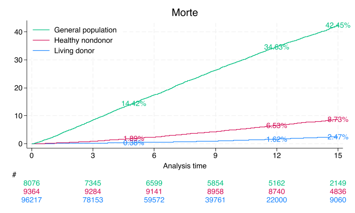
	ti("Morte")  
	text(`don5y' 5 "`don5y'%", col(stc1))  
	text(`don12y' 12 "`don12y'%", col(stc1))  
	text(`don15y' 15 "`don15y'%", col(stc1))  
	text(`hnd5y' 5 "`hnd5y'%", col(stc2))  
	text(`hnd12y' 12 "`hnd12y'%", col(stc2)) 
	text(`hnd15y' 15 "`hnd15y'%", col(stc2))  
	text(`gpop5y' 5 "`gpop5y'%", col(stc3))  
	text(`gpop12y' 12 "`gpop12y'%", col(stc3))  
	text(`gpop15y' 15 "`gpop15y'%", col(stc3));
#delimit cr

graph export ~/documents/github/work/jamascript.png, replace 
keep _* entry age_t0 female race donor
rename age_t0 age
//dataset
save ~/documents/github/work/jamascript.dta, replace 
noi stcox i.donor, basesurv(s0)
noi list s0 _t donor in 1/10
matrix define b=e(b)
keep s0 _t 
//s0
sort _t s0
list in 1/10
save ~/documents/github/work/s0.dta, replace 
export delimited using ~/documents/github/work/s0.csv, replace 
matrix beta = e(b)
svmat beta 
keep beta*
drop if missing(beta1)
//betas
list 
save b.dta, replace 
export delimited using ~/documents/github/work/b.csv, replace 
log close 
//noi ls
} 
 

        Failure _d: rSMGJcEdF_d==2
  Analysis time _t: (rSMGJcEdF_tT-origin)/365.25
            Origin: time rSMGJcEdF_t0

Iteration 0:  Log likelihood = -54332.522
Iteration 1:  Log likelihood =  -52993.14
Iteration 2:  Log likelihood = -51472.516
Iteration 3:  Log likelihood = -49543.907
Iteration 4:  Log likelihood =  -49520.68
Iteration 5:  Log likelihood = -49520.548
Iteration 6:  Log likelihood = -49520.548
Refining estimates:
Iteration 0:  Log likelihood = -49520.548

Cox regression with Breslow method for ties

No. of subjects =     113,657                          Number of obs = 113,657
No. of failures =       4,937
Time at risk    = 999,633.484
                                                       LR chi2(2)    = 9623.95
Log likelihood = -49520.548                            Prob > chi2   =  0.0000

-------------------------------------------------------------------------------
           _t | Haz. ratio   Std. err.      z    P>|z|     [95% conf. interval]
--------------+----------------------------------------------------------------
        donor |
HealthyNon~r  |   4.341779   .2130915    29.92   0.000     3.943586    4.780178
NotSoHealt~r  |   26.88098   1.007964    87.78   0.000     24.97625    28.93096
-------------------------------------------------------------------------------

     +-------------------------------+
     |        s0          _t   donor |
     |-------------------------------|
  1. | .98566928   11.277207   Donor |
  2. | .99256749   6.8281999   Donor |
  3. | .99351642   6.1711157   Donor |
  4. | .99402483   5.6919918   Donor |
  5. | .98475171   11.816564   Donor |
     |-------------------------------|
  6. | .99934972   .90622861   Donor |
  7. | .98705221   10.472279   Donor |
  8. |  .9879412   9.8754278   Donor |
  9. | .98766713   10.064339   Donor |
 10. | .99994059   .08761123   Donor |
     +-------------------------------+

Segev, JAMA, 2010:

• Page 961

• 5-year followup: \(0.4%\)

• 12-year follow-up: \(1.5%\)

Semiparametric

\(Y = \beta_0 + \beta_1X_1 + \beta_2X_2\)

\(\begin{bmatrix} \beta_0 \\ \beta_1 \\ \beta_2 \\ \vdots \\ \beta_N \end{bmatrix}\)

Where \(Y\) is the logHR:

• \(\beta_0\) is the logHR for living donors (the base-case & so equal to \(zero\))

• \(\beta_1\) is the logHR comparing nondonors to donors; thus \(X_1\) is the nondonor indicator

• \(\beta_2\) is the logHR comparing the general population to donors; thus \(X_2\) is the general population indicator

The \(\beta_i\) coeffients from the above Cox Regression can be found here

And the nonparametric base-case survival function can be found here

Show code cell source Hide code cell source

qui {
global repo https://github.com/abikesa/flow/raw/main/
import delimited "${repo}b.csv", clear 
rename (beta1 beta2 beta3)(donor nondonor genpop)
mkmat donor nondonor genpop, matrix(b)
matrix list b
matrix define SV = (1, 0, 0) 
matrix loghr = SV*b'
import delimited "${repo}s0.csv", clear
g f0 = (1 - s0)*100
g f1 = f0*exp(loghr[1,1])
sum f1 if _t < 12
//Segev, JAMA, 2010
noi di "Donor mortality at 12-year follow-up:" %3.2f r(max) "%" 
#delimit;
line f1 _t if inrange(_t,1,15), 
    sort 
	connect(step step) 
	ylab(0(10)40, 
	    format(%2.0f)
	) 
	xlab(0(3)15)
	yti("%")
	xti("Years")
	;
#delimit cr
}

Donor mortality at 12-year follow-up:1.55%