
#
#
Python#
Mixed Effects#
Objective:
The purpose of this assignment is to develop your understanding and skills in handling nested, hierarchical, multilevel, and longitudinal data structures. You will analyze a dataset that exhibits these characteristics using Python and relevant libraries such as pandas and statsmodels.
Dataset:
You are provided with a dataset (stsrpos.csv) containing information about medication prescriptions across various patients and time periods. The columns include:
usrds_id: The ID of the user/patient.gnn: The generic name of the medication.srvc_dt: The service date of the prescription.
Instructions:
Data Preparation:
Load the dataset and inspect its structure.
Convert the
srvc_dtcolumn to a proper date format.Create a new column representing the year and month of the service date.
Descriptive Analysis:
Calculate and visualize the distribution of prescriptions over time.
Identify the most frequently prescribed medications.
Hierarchical Data Analysis:
The data is inherently hierarchical with patients nested within prescription dates.
Determine the number of unique patients and prescriptions in the dataset.
Explore the variability in the number of prescriptions per patient over time.
Longitudinal Data Analysis:
Select a subset of patients who have at least five prescriptions over the observation period.
Examine how the frequency of their prescriptions changes over time.
Plot these changes for at least three selected patients to visualize their prescription trends.
Multilevel Modeling:
Build a simple linear mixed-effects model to predict the frequency of prescriptions using a random intercept for patients.
Interpret the results, focusing on the significance of the random effect.
Discussion:
Discuss the challenges and insights of working with hierarchical and longitudinal data.
Reflect on how multilevel modeling can help address issues of data dependency.
Submission:
Submit a Jupyter notebook containing all code, outputs, visualizations, and a discussion. Make sure to clearly comment your code and provide insightful interpretations of your results.
1. Data Preparation:
Load the dataset and inspect its structure:
import pandas as pd
import requests

# Correct URL
url = 'https://github.com/jhustata/lab6.md/raw/main/stsrpos.csv'
response = requests.get(url)
response.raise_for_status()  # Raise an error for bad status codes

# Save the content to a temporary file
with open('temp_stsrpos.csv', 'wb') as temp_file:
    temp_file.write(response.content)

# Load the dataset from the temporary file
dataset = pd.read_csv('temp_stsrpos.csv')

# Display the first few rows and column names
dataset.head(), dataset.columns
(   usrds_id                        gnn    srvc_dt
 0         0                 FEBUXOSTAT  11oct2024
 1         1        CYCLOBENZAPRINE HCL  15jun2024
 2         7       LEVOTHYROXINE SODIUM  18feb2024
 3        12             INSULIN ASPART  17nov2024
 4        15  HYDROCODONE/ACETAMINOPHEN  14jan2024,
 Index(['usrds_id', 'gnn', 'srvc_dt'], dtype='object'))
import pandas as pd

dataset = pd.read_csv('temp_stsrpos.csv')
dataset.head()
| usrds_id | gnn | srvc_dt | |
|---|---|---|---|
| 0 | 0 | FEBUXOSTAT | 11oct2024 |
| 1 | 1 | CYCLOBENZAPRINE HCL | 15jun2024 |
| 2 | 7 | LEVOTHYROXINE SODIUM | 18feb2024 |
| 3 | 12 | INSULIN ASPART | 17nov2024 |
| 4 | 15 | HYDROCODONE/ACETAMINOPHEN | 14jan2024 |
Convert
srvc_dtcolumn to a proper date format:
Create a new column for the year and month:
dataset['srvc_dt'] = pd.to_datetime(dataset['srvc_dt'], format='%d%b%Y')
dataset['year_month'] = dataset['srvc_dt'].dt.to_period('M')
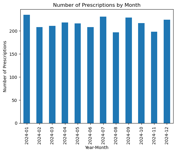
2. Descriptive Analysis:
Calculate and visualize the distribution of prescriptions over time:
import matplotlib.pyplot as plt

# Count prescriptions by month
month_counts = dataset['year_month'].value_counts().sort_index()

# Plotting
month_counts.plot(kind='bar', title='Number of Prescriptions by Month')
plt.ylabel('Number of Prescriptions')
plt.xlabel('Year-Month')
plt.show()
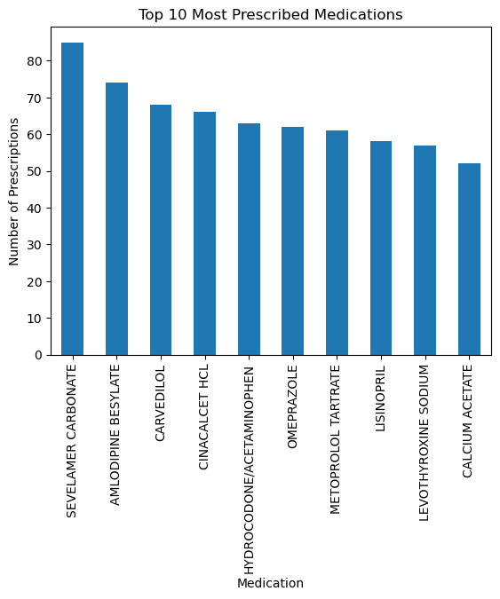
Identify the most frequently prescribed medications:
top_meds = dataset['gnn'].value_counts().head(10)
top_meds.plot(kind='bar', title='Top 10 Most Prescribed Medications')
plt.ylabel('Number of Prescriptions')
plt.xlabel('Medication')
plt.show()
3. Hierarchical Data Analysis:
Determine the number of unique patients and prescriptions:
num_patients = dataset['usrds_id'].nunique()
num_prescriptions = len(dataset)
Explore the variability in the number of prescriptions per patient:
prescriptions_per_patient = dataset['usrds_id'].value_counts()
prescriptions_per_patient.describe()
count    2271.000000
mean        1.141347
std         0.383370
min         1.000000
25%         1.000000
50%         1.000000
75%         1.000000
max         4.000000
Name: usrds_id, dtype: float64
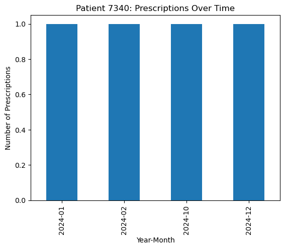
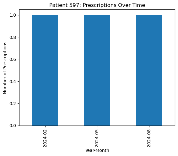
4. Longitudinal Data Analysis:
Select a subset of patients with at least three prescriptions:
patients_with_3_plus = prescriptions_per_patient[prescriptions_per_patient >= 3].index
subset = dataset[dataset['usrds_id'].isin(patients_with_3_plus)]
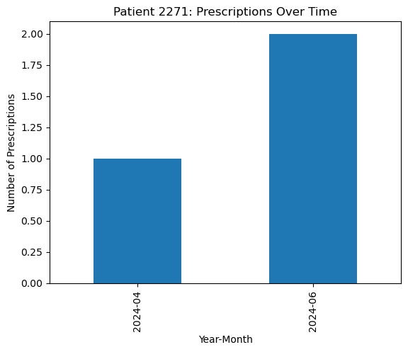
Examine and plot the frequency of prescriptions over time for selected patients:
selected_patients = patients_with_3_plus[:3]

for patient_id in selected_patients:
    patient_data = subset[subset['usrds_id'] == patient_id]
    freq_over_time = patient_data['year_month'].value_counts().sort_index()
    freq_over_time.plot(kind='bar', title=f'Patient {patient_id}: Prescriptions Over Time')
    plt.ylabel('Number of Prescriptions')
    plt.xlabel('Year-Month')
    plt.show()
5. Multilevel Modeling:
Build a linear mixed-effects model:
import statsmodels.formula.api as smf
import pandas as pd

# Convert 'year_month' to string
dataset['year_month'] = dataset['year_month'].astype(str)

# Fit the mixed-effects model
model = smf.mixedlm("usrds_id ~ year_month", dataset, groups=dataset["usrds_id"])
result = model.fit()
print(result.summary())
                   Mixed Linear Model Regression Results
============================================================================
Model:                   MixedLM       Dependent Variable:       usrds_id
No. Observations:        2592          Method:                   REML
No. Groups:              2271          Scale:                    0.0316
Min. group size:         1             Log-Likelihood:           -21180.9335
Max. group size:         4             Converged:                Yes
Mean group size:         1.1
----------------------------------------------------------------------------
                         Coef.      Std.Err.    z    P>|z|  [0.025   0.975]
----------------------------------------------------------------------------
Intercept                4966.686      56.473 87.948 0.000 4856.001 5077.371
year_month[T.2024-02]      -0.000       0.048 -0.000 1.000   -0.093    0.093
year_month[T.2024-03]       0.000       0.050  0.000 1.000   -0.098    0.098
year_month[T.2024-04]       0.000       0.048  0.000 1.000   -0.095    0.095
year_month[T.2024-05]       0.000       0.050  0.000 1.000   -0.098    0.098
year_month[T.2024-06]       0.000       0.049  0.000 1.000   -0.096    0.096
year_month[T.2024-07]       0.000       0.048  0.000 1.000   -0.094    0.094
year_month[T.2024-08]      -0.000       0.053 -0.000 1.000   -0.104    0.104
year_month[T.2024-09]       0.000       0.050  0.000 1.000   -0.099    0.099
year_month[T.2024-10]       0.000       0.052  0.000 1.000   -0.103    0.103
year_month[T.2024-11]      -0.000       0.053 -0.000 1.000   -0.104    0.104
year_month[T.2024-12]       0.000       0.051  0.000 1.000   -0.100    0.100
Group Var             7242677.078 3273083.158
============================================================================
The model here is quite simple and is mostly for illustrative purposes. The TA can expect variations, such as different covariates in the formula or more complex structures for the random effects.
6. Discussion:
This section is primarily qualitative, but TAs should encourage students to discuss:
The hierarchical nature of the data.
The use of multilevel modeling to account for nested data structures.
The challenges of longitudinal data, such as missing data and varying observation times.
The insights gained from the analysis and how it informed their understanding of the dataset.
By providing these solutions and hints, TAs should be able to effectively guide students through the assignment while allowing flexibility for different approaches and interpretations.
This output is from a mixed linear model (MLM) regression analysis. Let’s break down the key parts:
Model Summary:
Model: MixedLM (Mixed Linear Model)
Dependent Variable: usrds_id
No. Observations: 2592
Method: REML (Restricted Maximum Likelihood)
No. Groups: 2271
Scale: 0.0316
Log-Likelihood: -21180.9335
Converged: Yes
Mean group size: 1.1
Coefficients:
Intercept: 4966.686, Std.Err. 56.473, z 87.948, P>|z| 0.000
year_month[T.2024-02] to year_month[T.2024-12]: These are the coefficients for each month of the year 2024. They all seem to be close to zero, with standard errors close to zero as well, and p-values of 1.000, indicating that these coefficients are not statistically significant.
Group Variance: 7242677.078, Std.Err. 3273083.158: This represents the variance between groups (different usrds_id), suggesting there is substantial variation between groups.
Overall, the model suggests that there is no significant relationship between the year_month and usrds_id variables. The intercept, which represents the average usrds_id, is the main factor influencing the dependent variable in this model.
3. society#
Please review abikesa/society for motivation
pip install --no-cache-dir geopandas
Show code cell source
import geopandas as gpd
import pandas as pd
import warnings
import geopandas.datasets
import matplotlib.pyplot as plt

# Load the world map shapefile from the downloaded file
world_path = '~/documents/github/myenv/lib/python3.11/site-packages/geopandas/datasets/naturalearth_lowres/naturalearth_lowres.shp'
world = gpd.read_file(world_path)

# Suppress FutureWarnings
warnings.simplefilter(action='ignore', category=FutureWarning)
Show code cell source
# Load the world map shapefile
world = gpd.read_file(gpd.datasets.get_path('naturalearth_lowres'))
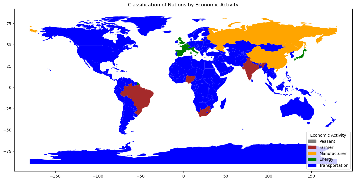
# GDP per capita data (example data, actual values would vary)
gdp_per_capita = {
'Austria': 52000, 'Belgium': 47500, 'Brazil': 9000, 'China': 11000,
'France': 43000, 'Germany': 52000, 'India': 2000, 'Italy': 40000,
'Japan': 42000, 'Nigeria': 2000, 'Russia': 11000, 'South Africa': 6500,
'Spain': 31000, 'Switzerland': 82000, 'United Kingdom': 43000, 'United States': 62000
}
# Classify countries
def classify_gdp_per_capita(gdp):
if gdp < 2000:
return 'Peasant'
elif 2000 <= gdp < 10000:
return 'Farmer'
elif 10000 <= gdp < 30000:
return 'Manufacturer'
elif 30000 <= gdp < 50000:
return 'Energy'
else:
return 'Transportation'
world['Economic_Classification'] = world['name'].map(gdp_per_capita).apply(classify_gdp_per_capita)
# Define colors for each classification
colors = {
'Peasant': 'gray',
'Farmer': 'brown',
'Manufacturer': 'orange',
'Energy': 'green',
'Transportation': 'blue'
}
# Plot the world map
fig, ax = plt.subplots(figsize=(15, 10))
world.plot(ax=ax, color=world['Economic_Classification'].map(colors))
# Add a legend
handles = [plt.Rectangle((0,0),1,1, color=colors[label]) for label in colors]
labels = colors.keys()
ax.legend(handles, labels, title='Economic Activity', loc='lower right')
plt.title('Classification of Nations by Economic Activity')
plt.show()
Show code cell source
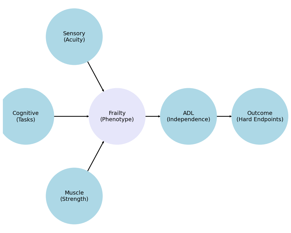
import networkx as nx
import matplotlib.pyplot as plt
G = nx.DiGraph()
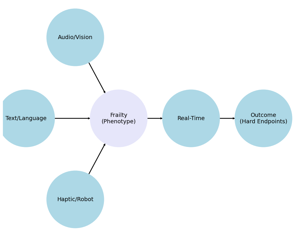
G.add_node("Audio/Vision", pos=(-2500, 700))
G.add_node("Text/Language", pos=(-4200, 0))
G.add_node("Frailty", pos=(-1000, 0))
G.add_node("Haptic/Robot", pos=(-2500, -700))
G.add_node("Real-Time", pos=(1500, 0))
G.add_node("Outcome", pos=(4000, 0))
G.add_edges_from([("Audio/Vision", "Frailty")])
G.add_edges_from([("Text/Language", "Frailty")])
G.add_edges_from([("Haptic/Robot", "Frailty")])
G.add_edges_from([("Frailty", "Real-Time")])
G.add_edges_from([("Real-Time", "Outcome")])
pos = nx.get_node_attributes(G, 'pos')
labels = {"Frailty": "Frailty\n(Phenotype)",
"Audio/Vision": "Audio/Vision",
"Text/Language": "Text/Language",
"Haptic/Robot": "Haptic/Robot",
"Real-Time": "Real-Time",
"Outcome": "Outcome\n(Hard Endpoints)"} # Added label for "NDI" node in the labels dictionary
# Update color for the "Scenarios" node
node_colors = ["lightblue","lightblue", "lavender", "lightblue", "lightblue", "lightblue"]
# node_colors = ["lightblue","lavender", "lavender", "lightgreen", "lightpink", "lightpink"]
# Suppress the deprecation warning
import warnings
warnings.filterwarnings("ignore", category=DeprecationWarning)
plt.figure(figsize=(10, 8))
nx.draw(G, pos, with_labels=False, node_size=20000, node_color=node_colors, linewidths=2, edge_color='black', style='solid')
nx.draw_networkx_labels(G, pos, labels, font_size=14) # , font_weight='bold'
nx.draw_networkx_edges(G, pos, edge_color='black', style='solid', width=2)
plt.xlim(-5000, 5000)
plt.ylim(-1000, 1000)
plt.axis("off")
plt.show()
import numpy as np
import matplotlib.pyplot as plt
from scipy import stats
import pandas as pd

# Extend the list of characteristics to 10
characteristics_extended = [
    "Percentage of Female-headed households",
    "Percentage of households with no car",
    "Percentage of households below poverty level",
    "Percentage of people unemployed",
    "Percentage of people with less than high school education",
    "Percentage of people on public assistance",
    "Percentage of people with disabilities",
    "Percentage of people who are renters",
    "Percentage of people who are immigrants",
    "Percentage of people who moved in the past year"
]

# Simulate hazard ratios for 10 characteristics
hazard_ratios_extended = np.random.uniform(0.5, 2.0, len(characteristics_extended))

# Calculate log hazard ratios
log_hazard_ratios_extended = np.log(hazard_ratios_extended)

# Simulate 95% CI for log hazard ratios (mean ± 1.96*standard error)
std_errors_extended = np.random.uniform(0.1, 0.3, len(characteristics_extended))
lower_ci_log_hr_extended = log_hazard_ratios_extended - 1.96 * std_errors_extended
upper_ci_log_hr_extended = log_hazard_ratios_extended + 1.96 * std_errors_extended

# Create the DataFrame
data_extended = {
    "Characteristic": characteristics_extended,
    "Hazard Ratio": hazard_ratios_extended,
    "Log Hazard Ratio": log_hazard_ratios_extended,
    "95% CI Lower (Log Hazard Ratio)": lower_ci_log_hr_extended,
    "95% CI Upper (Log Hazard Ratio)": upper_ci_log_hr_extended
}

df_extended = pd.DataFrame(data_extended)

# Display the DataFrame
print(df_extended)
                                      Characteristic  Hazard Ratio  \
0             Percentage of Female-headed households      0.774819
1               Percentage of households with no car      0.648893
2       Percentage of households below poverty level      1.971006
3                    Percentage of people unemployed      0.936912
4  Percentage of people with less than high schoo...      1.260453
5          Percentage of people on public assistance      1.692673
6             Percentage of people with disabilities      0.666209
7               Percentage of people who are renters      0.778261
8            Percentage of people who are immigrants      1.735064
9    Percentage of people who moved in the past year      1.399486

   Log Hazard Ratio  95% CI Lower (Log Hazard Ratio)  \
0         -0.255126                        -0.502808
1         -0.432488                        -0.675031
2          0.678544                         0.253230
3         -0.065166                        -0.461516
4          0.231471                        -0.307911
5          0.526309                         0.083652
6         -0.406152                        -0.663905
7         -0.250694                        -0.696921
8          0.551044                         0.344570
9          0.336105                        -0.154140

   95% CI Upper (Log Hazard Ratio)
0                        -0.007443
1                        -0.189945
2                         1.103858
3                         0.331185
4                         0.770854
5                         0.968966
6                        -0.148398
7                         0.195534
8                         0.757519
9                         0.826350
import numpy as np
import matplotlib.pyplot as plt
from scipy import stats
import pandas as pd
import pandas as pd
import requests
from io import StringIO
url = "https://github.com/abikesa/format/raw/main/donor_live.csv"
response = requests.get(url)
if response.status_code == 200:
csv_data = StringIO(response.text)
df = pd.read_csv(csv_data)
print(df.head())
else:
print(f"Failed to download file, status code: {response.status_code}")
# Print DataFrame info to verify load
print(df.info())
# Clean and convert data types
df['pers_id'] = pd.to_numeric(df['pers_id'], errors='coerce')
df['don_age_in_months'] = pd.to_numeric(df['don_age_in_months'], errors='coerce')
df['don_age'] = pd.to_numeric(df['don_age'], errors='coerce')
df['don_race'] = pd.to_numeric(df['don_race'], errors='coerce')
# Display basic statistics for continuous variables
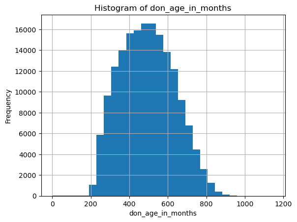
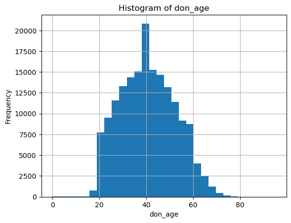
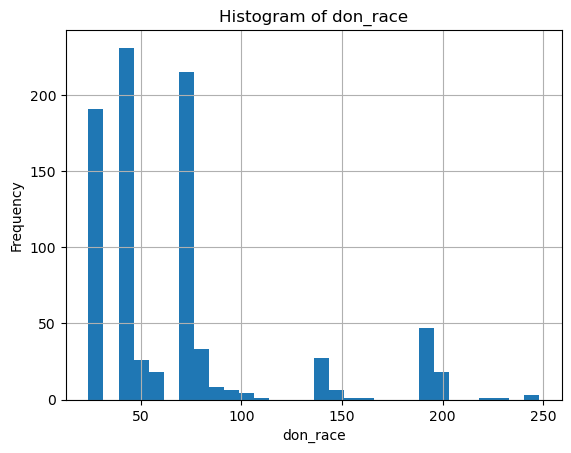
print(df[['don_age_in_months', 'don_age', 'don_race']].describe())
# Plot histograms for continuous variables
continuous_vars = ['don_age_in_months', 'don_age', 'don_race']
for var in continuous_vars:
plt.figure()
df[var].dropna().hist(bins=30)
plt.title(f'Histogram of {var}')
plt.xlabel(var)
plt.ylabel('Frequency')
plt.show()
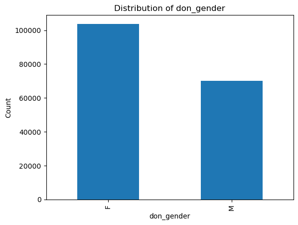
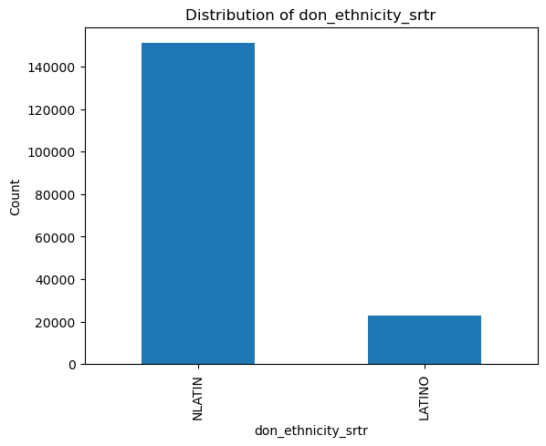
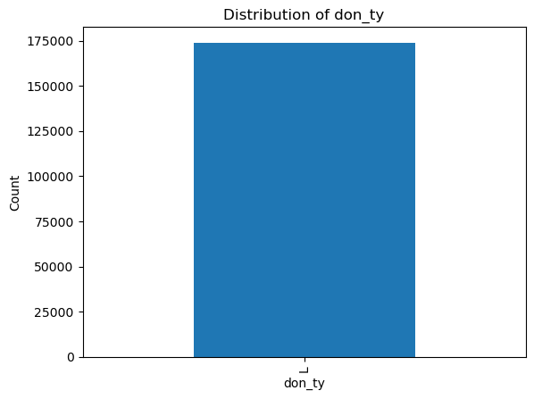
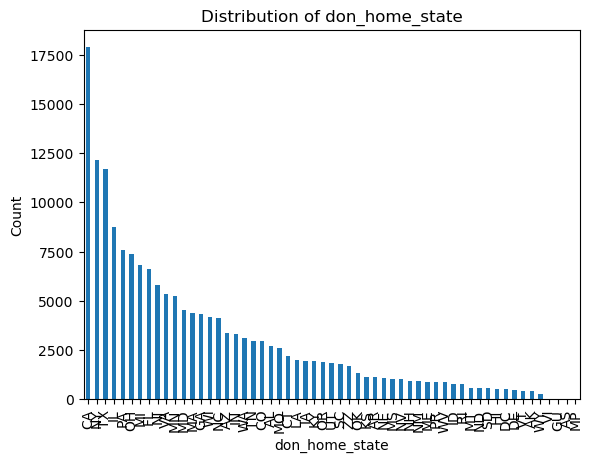
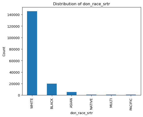
# Count and plot binary/categorical variables
binary_vars = ['don_gender', 'don_ethnicity_srtr']
categorical_vars = ['don_ty', 'don_home_state', 'don_race_srtr']
for var in binary_vars + categorical_vars:
plt.figure()
df[var].value_counts().plot(kind='bar')
plt.title(f'Distribution of {var}')
plt.xlabel(var)
plt.ylabel('Count')
plt.show()
   don_id  pers_id don_ty  don_age_in_months  don_age don_gender  \
0  HRG962      289      L              490.0     40.0          F
1  IT5273      484      L              312.0     26.0          F
2  HRL860      840      L              648.0     54.0          M
3  ZWB847      967      L              564.0     47.0          M
4  ALB852     1145      L              326.0     27.0          F

  don_home_state  don_ethnicity_pre2004  don_race_pre2004  \
0             TX                    2.0               8.0
1             OH                    2.0               8.0
2             ND                    2.0               8.0
3             NY                    1.0               8.0
4             CA                    1.0               8.0

                        don_race  ... don_hyperten_postop  \
0                       8: White  ...                   N
1                       8: White  ...                   N
2                       8: White  ...                   N
3          2000: Hispanic/Latino  ...                 NaN
4          2000: Hispanic/Latino  ...                 NaN

  pers_esrd_first_service_dt  pers_esrd_first_dial_dt  pers_esrd_ki_dgn  \
0                        NaN                      NaN               NaN
1                        NaN                      NaN               NaN
2                        NaN                      NaN               NaN
3                        NaN                      NaN               NaN
4                        NaN                      NaN               NaN

   don_race_american_indian don_race_asian don_race_black_african_american  \
0                         0              0                               0
1                         0              0                               0
2                         0              0                               0
3                         0              0                               0
4                         0              0                               0

  don_race_hispanic_latino don_race_native_hawaiian don_race_white
0                        0                        0              1
1                        0                        0              1
2                        0                        0              1
3                        1                        0              0
4                        1                        0              0

[5 rows x 36 columns]
<class 'pandas.core.frame.DataFrame'>
RangeIndex: 173929 entries, 0 to 173928
Data columns (total 36 columns):
 #   Column                           Non-Null Count   Dtype
---  ------                           --------------   -----
 0   don_id                           173929 non-null  object
 1   pers_id                          173929 non-null  int64
 2   don_ty                           173929 non-null  object
 3   don_age_in_months                173922 non-null  float64
 4   don_age                          173922 non-null  float64
 5   don_gender                       173929 non-null  object
 6   don_home_state                   170492 non-null  object
 7   don_ethnicity_pre2004            131260 non-null  float64
 8   don_race_pre2004                 131260 non-null  float64
 9   don_race                         173851 non-null  object
 10  don_race_srtr                    173815 non-null  object
 11  don_ethnicity_srtr               173929 non-null  object
 12  don_home_country                 0 non-null       float64
 13  don_hgt_cm                       130924 non-null  float64
 14  don_wgt_kg                       132825 non-null  float64
 15  don_recov_dt                     173929 non-null  object
 16  don_relationship_ty              172919 non-null  object
 17  don_diab                         101127 non-null  object
 18  don_hyperten_diet                3283 non-null    object
 19  don_hyperten_diuretics           3283 non-null    object
 20  don_hyperten_other_meds          3283 non-null    object
 21  don_ki_creat_preop               128276 non-null  float64
 22  don_bp_preop_syst                118935 non-null  float64
 23  don_bp_preop_diast               118915 non-null  float64
 24  pers_esrd_death_dt               79 non-null      float64
 25  pers_ssa_death_dt                1395 non-null    object
 26  don_hyperten_postop              101066 non-null  object
 27  pers_esrd_first_service_dt       706 non-null     float64
 28  pers_esrd_first_dial_dt          690 non-null     float64
 29  pers_esrd_ki_dgn                 332 non-null     float64
 30  don_race_american_indian         173929 non-null  int64
 31  don_race_asian                   173929 non-null  int64
 32  don_race_black_african_american  173929 non-null  int64
 33  don_race_hispanic_latino         173929 non-null  int64
 34  don_race_native_hawaiian         173929 non-null  int64
 35  don_race_white                   173929 non-null  int64
dtypes: float64(14), int64(7), object(15)
memory usage: 47.8+ MB
None
       don_age_in_months        don_age    don_race
count      173922.000000  173922.000000  838.000000
mean          493.620244      40.676142   65.250597
std           139.174427      11.600951   48.149922
min             0.000000       0.000000   24.000000
25%           385.000000      32.000000   40.000000
50%           489.000000      40.000000   40.000000
75%           595.000000      49.000000   72.000000
max          1151.000000      95.000000  248.000000
GPT-4o suggests python load_csv.py#
You’re welcome! If you need to use the requests library to fetch the CSV file because pandas is having trouble directly accessing it, the code provided should work well for you. Here’s a recap of the complete solution for your setup in VSCode on a Mac:
Set up a Python environment:
Open your terminal in VSCode and create a virtual environment:
python3 -m venv myenv
source myenv/bin/activate  # On Windows, use `myenv\Scripts\activate`
Install the required libraries:
Ensure you have
pandasandrequestsinstalled:pip install pandas requests
Create and run your Python script:
Create a new Python file, for example,
load_csv.py, and add the following code:import pandas as pd import requests from io import StringIO url = "https://github.com/abikesa/format/raw/main/donor_live.csv" response = requests.get(url) if response.status_code == 200: csv_data = StringIO(response.text) df = pd.read_csv(csv_data) print(df.head()) else: print(f"Failed to download file, status code: {response.status_code}")
Run the script:
In the VSCode terminal, make sure your virtual environment is activated, and then run:
python load_csv.py
This will download the CSV file using requests, read it into a pandas DataFrame, and print the first few rows. If everything is set up correctly, you should see the data printed in the terminal.
If you encounter any issues or have further questions, feel free to ask!