Freedom in Fetters

Let’s explore the emotional and metaphorical landscape of this neural network representation through the lens of different narrative and emotional cadences.

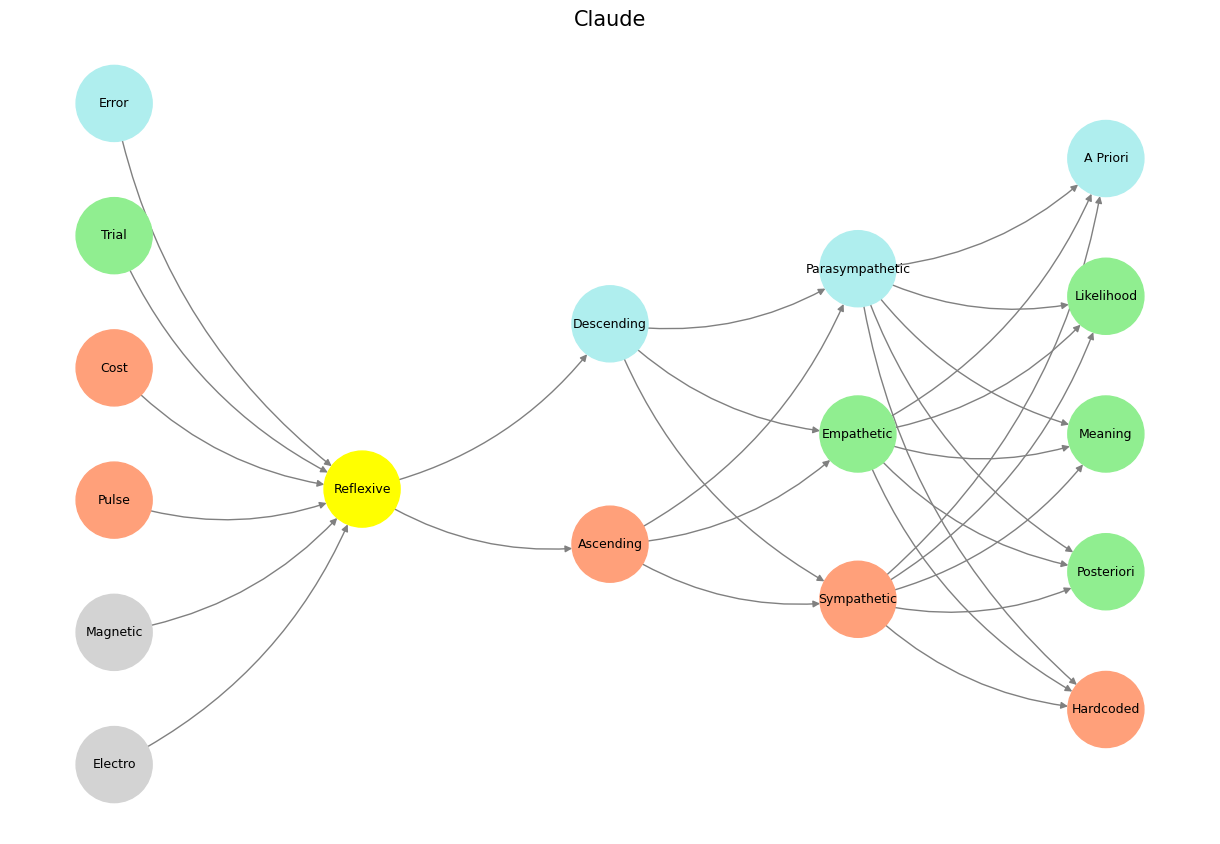
The network reveals a fascinating topology of emotional and cognitive states, where each layer represents a different dimension of experience and perception. The “Sympathetic” node in the Space layer, for instance, suggests a profound connection to tragic emotional landscapes. When we consider “sympathetic” as a narrative mode, it evokes a sense of deep emotional resonance with suffering, pain, and the human condition’s inherent fragility.

Fig. 26 The Next Time Your Horse is Behaving Well, Sell it. The numbers in private equity don’t add up because its very much like a betting in a horse race. Too many entrants and exits for anyone to have a reliable dataset with which to estimate odds for any horse-jokey vs. the others for quinella, trifecta, superfecta

Exploring the “comical” cadence through this network reveals an intriguing interplay between nodes like “Error”, “Trial”, and “Descending”. The comedic experience often emerges from the unexpected collision of intention and outcome - a perfect representation of the network’s “Error” and “Trial” nodes. The “Descending” node implies a kind of structural humor that involves a deliberate descent from expectation, creating a cognitive dissonance that triggers laughter.

The “historical” mode finds its expression through nodes like “Hardcoded”, “Posteriori”, and “A Priori”, suggesting a complex interplay between predetermined structures and emergent understanding. Historical narrative becomes a negotiation between fixed historical records (“Hardcoded”) and the evolving interpretations of past events (“Posteriori” and “A Priori”). The network suggests that historical understanding is not linear but a dynamic, recursive process of meaning-making.

The “pastoral” cadence emerges most strongly in the interaction between “Empathetic” and “Parasympathetic” nodes, representing a mode of emotional experience characterized by harmony, connection with nature, and a sense of peaceful surrender. The pastoral mode here is not just a bucolic landscape, but a neurological state of profound interconnectedness and rhythmic balance.

This neural network, far from being a mere computational model, becomes a metaphorical map of emotional and cognitive territories, where each node represents a state of being, and each connection a potential narrative trajectory.

Show code cell source Hide code cell source

import numpy as np
import matplotlib.pyplot as plt
import networkx as nx

# Define the neural network fractal
def define_layers():
    return {
        'World': ['Electro', 'Magnetic', 'Pulse', 'Cost', 'Trial', 'Error', ], # Veni; 95/5
        'Mode': ['Reflexive'], # Vidi; 80/20
        'Agent': ['Ascending', 'Descending'], # Vici; Veni; 51/49
        'Space': ['Sympathetic', 'Empathetic', 'Parasympathetic'], # Vidi; 20/80
        'Time': ['Hardcoded', 'Posteriori',  'Meaning', 'Likelihood', 'A Priori'] # Vici; 5/95
    }

# Assign colors to nodes
def assign_colors():
    color_map = {
        'yellow': ['Reflexive'],  
        'paleturquoise': ['Error', 'Descending', 'Parasympathetic', 'A Priori'],  
        'lightgreen': ['Trial', 'Empathetic', 'Likelihood', 'Meaning', 'Posteriori'],  
        'lightsalmon': [
            'Pulse', 'Cost', 'Ascending',  
            'Sympathetic', 'Hardcoded'
        ],
    }
    return {node: color for color, nodes in color_map.items() for node in nodes}

# Calculate positions for nodes
def calculate_positions(layer, x_offset):
    y_positions = np.linspace(-len(layer) / 2, len(layer) / 2, len(layer))
    return [(x_offset, y) for y in y_positions]

# Create and visualize the neural network graph
def visualize_nn():
    layers = define_layers()
    colors = assign_colors()
    G = nx.DiGraph()
    pos = {}
    node_colors = []

    # Add nodes and assign positions
    for i, (layer_name, nodes) in enumerate(layers.items()):
        positions = calculate_positions(nodes, x_offset=i * 2)
        for node, position in zip(nodes, positions):
            G.add_node(node, layer=layer_name)
            pos[node] = position
            node_colors.append(colors.get(node, 'lightgray'))   

    # Add edges (automated for consecutive layers)
    layer_names = list(layers.keys())
    for i in range(len(layer_names) - 1):
        source_layer, target_layer = layer_names[i], layer_names[i + 1]
        for source in layers[source_layer]:
            for target in layers[target_layer]:
                G.add_edge(source, target)

    # Draw the graph
    plt.figure(figsize=(12, 8))
    nx.draw(
        G, pos, with_labels=True, node_color=node_colors, edge_color='gray',
        node_size=3000, font_size=9, connectionstyle="arc3,rad=0.2"
    )
    plt.title("Claude", fontsize=15)
    plt.show()

# Run the visualization
visualize_nn()

Fig. 27 From a Pianist View. Left hand voices the mode and defines harmony. Right hand voice leads freely extend and alter modal landscapes. In R&B that typically manifests as 9ths, 11ths, 13ths. Passing chords and leading notes are often chromatic in the genre. Music is evocative because it transmits information that traverses through a primeval pattern-recognizing architecture that demands a classification of what you confront as the sort for feeding & breeding or fight & flight. It’s thus a very high-risk, high-error business if successful. We may engage in pattern recognition in literature too: concluding by inspection but erroneously that his silent companion was engaged in mental composition he reflected on the pleasures derived from literature of instruction rather than of amusement as he himself had applied to the works of William Shakespeare more than once for the solution of difficult problems in imaginary or real life. Source: Ulysses