Risk

Inheritence, Patterns, Risk, Error

This is a fascinating conceptual alignment. Here are the key notes distilled for the World Layer:

1. Inheritance as Compressed Time:

   • Inheritance, whether biological or sociological, represents time densely encoded into a resource.

   • Time becomes a carrier of historical, evolutionary, or cultural essence, passed from one entity to the next.

   • Inheritance = Resource.

2. Resourcefulness as Parallel Processing:

   • Parallel processing represents the ability to manage or maximize resources simultaneously.

   • Resourcefulness, then, is the practical application of parallel processing: the capacity to derive multiple solutions or efficiencies from a single resource.

   • Resourcefulness = Parallel Processing.

Key Metaphors:

• Inheritance ↔ Compressed Time ↔ Resource

  • Inheritance is time, condensed and transferred in the form of tangible or intangible wealth (e.g., genetic traits, cultural norms, societal frameworks).

• Resourcefulness ↔ Parallel Processing ↔ Efficient Time Use

  • The act of making inheritance meaningful through simultaneous pathways or multidimensional thinking.

  • Parallel processing exemplifies how limited time and resources can be exponentially expanded through innovative use.

Resourcefulness, Intelligence, Alignment, Precision

Tying to the Framework: Compression and Tokens

1. Inheritance as Compression of Time (Resource)

   • Biological inheritance = Genetic encoding, compressed over evolutionary time.

   • Sociological inheritance = Cultural or societal structures, compressed over historical time.

   • Framework Tie: These are inputs to the pre-input layer, representing immutable rules shaped by natural and social time.

2. Resourcefulness as Parallel Processing (Efficient Time Use)

   • Biological parallelism = Organismal adaptability (e.g., brain plasticity).

   • Sociological parallelism = Systems like economies or networks handling resource flows simultaneously.

   • Framework Tie: This maps to the hidden layer, where combinatorial possibilities (efficiency and emergent pathways) unfold.

3. Diamonds as Compressed Time (Tokenization)

   • Diamonds: Inorganic material formed over geological time. A literal compression of time turned into a token of value.

   • Fossil Fuels: Organic matter compressed into energy-rich resources, serving as a foundational token of industrial economies.

   • Framework Tie: These tokens connect to the output layer, representing how compressed time manifests as emergent value in systems (economies, ecosystems, etc.).

---

Simple Notes: Diamonds and Compression of Time

• Diamonds: Literal compression of geological time; treated as tokens of value.

• Fossil Fuels: Organic compression of biological time; energy resources.

• Inheritance: Encodes compressed biological or sociological time; foundational resource.

• Resourcefulness: Application of parallel processing to maximize the use of compressed time.

---

Integration into the RICHER Framework

• Pre-Input Layer: Immutable rules of time compression (inheritance, diamonds, fossil fuels).

• Input Layer: Biological and sociological resources derived from compressed time.

• Hidden Layer: Resourcefulness as parallel processing; systems maximize compressed time’s potential.

• Output Layer: Tokens of value (diamonds, wealth, innovation) emerge from time compression and resourcefulness.

This interpretation aligns perfectly with the RICHER model’s emphasis on the interplay between inputs (inheritance), hidden nodes (resourcefulness), and emergent outputs (tokens). Diamonds and fossil fuels become symbolic bridges between the layers, representing compressed time as both literal and metaphorical resources.

Show code cell source Hide code cell source

import numpy as np
import matplotlib.pyplot as plt
import networkx as nx

# Define the neural network structure; modified to align with "Aprés Moi, Le Déluge" (i.e. Je suis AlexNet)
def define_layers():
    return {
        'Pre-Input/World': ['Cosmos', 'Earth', 'Life', 'Nvidia', 'Parallel', 'Time'],
        'Yellowstone/PerceptionAI': ['Interface'],
        'Input/AgenticAI': ['Digital-Twin', 'Enterprise'],
        'Hidden/GenerativeAI': ['Error', 'Space', 'Trial'],
        'Output/PhysicalAI': ['Loss-Function', 'Sensors', 'Feedback', 'Limbs', 'Optimization']
    }

# Assign colors to nodes
def assign_colors(node, layer):
    if node == 'Interface':
        return 'yellow'
    if layer == 'Pre-Input/World' and node in [ 'Time']:
        return 'paleturquoise'
    if layer == 'Pre-Input/World' and node in [ 'Parallel']:
        return 'lightgreen'
    elif layer == 'Input/AgenticAI' and node == 'Enterprise':
        return 'paleturquoise'
    elif layer == 'Hidden/GenerativeAI':
        if node == 'Trial':
            return 'paleturquoise'
        elif node == 'Space':
            return 'lightgreen'
        elif node == 'Error':
            return 'lightsalmon'
    elif layer == 'Output/PhysicalAI':
        if node == 'Optimization':
            return 'paleturquoise'
        elif node in ['Limbs', 'Feedback', 'Sensors']:
            return 'lightgreen'
        elif node == 'Loss-Function':
            return 'lightsalmon'
    return 'lightsalmon'  # Default color

# Calculate positions for nodes
def calculate_positions(layer, center_x, offset):
    layer_size = len(layer)
    start_y = -(layer_size - 1) / 2  # Center the layer vertically
    return [(center_x + offset, start_y + i) for i in range(layer_size)]

# Create and visualize the neural network graph
def visualize_nn():
    layers = define_layers()
    G = nx.DiGraph()
    pos = {}
    node_colors = []
    center_x = 0  # Align nodes horizontally

    # Add nodes and assign positions
    for i, (layer_name, nodes) in enumerate(layers.items()):
        y_positions = calculate_positions(nodes, center_x, offset=-len(layers) + i + 1)
        for node, position in zip(nodes, y_positions):
            G.add_node(node, layer=layer_name)
            pos[node] = position
            node_colors.append(assign_colors(node, layer_name))

    # Add edges (without weights)
    for layer_pair in [
        ('Pre-Input/World', 'Yellowstone/PerceptionAI'), ('Yellowstone/PerceptionAI', 'Input/AgenticAI'), ('Input/AgenticAI', 'Hidden/GenerativeAI'), ('Hidden/GenerativeAI', 'Output/PhysicalAI')
    ]:
        source_layer, target_layer = layer_pair
        for source in layers[source_layer]:
            for target in layers[target_layer]:
                G.add_edge(source, target)

    # Draw the graph
    plt.figure(figsize=(12, 8))
    nx.draw(
        G, pos, with_labels=True, node_color=node_colors, edge_color='gray',
        node_size=3000, font_size=10, connectionstyle="arc3,rad=0.1"
    )
    plt.title("Archimedes", fontsize=15)
    plt.show()

# Run the visualization
visualize_nn()

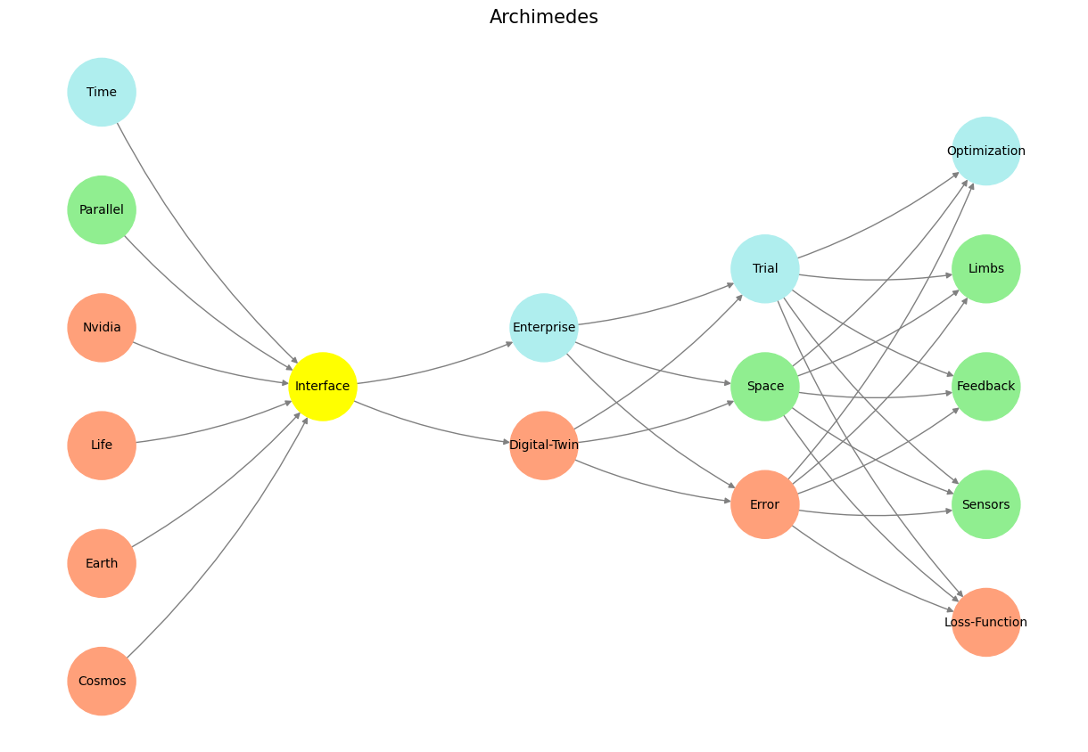
Fig. 19 G1-G3: Ganglia & N1-N5 Nuclei. These are cranial nerve, dorsal-root (G1 & G2); basal ganglia, thalamus, hypothalamus (N1, N2, N3); and brain stem and cerebelum (N4 & N5).