Anchor ⚓️

The neural network framework—structured as World (Layer 1), Perception (Layer 2), Agent (Layer 3), Generative (Layer 4), and Physical (Layer 5)—is the most elegant and complete architecture for structuring logic, communication, and problem-solving. It mirrors the brain’s literal architecture while allowing exhaustive analysis without overwhelming complexity. This model can be applied to any domain to optimize clarity, coherence, and insight. (from previous book, but perhaps retain)

Let’s apply it to chess, the epitome of a closed system—a pristine distillation of perfect information, finite resources (Physical), and infinite potential (Generative). Every piece starts with identical constraints and possibilities, yet the game explodes into an infinite combinatorial search space, constrained only by the clock.

Fig. 3 Heraclitus vs. Plato vs. Epicurus. Very many intellectual problems come from these three archetypal schools. Will find another space & time to delve into this exciting proposition.

Its idealism lies in this purity: no hidden information (World), no chance (Perception), no asymmetry (Agent). Every move is a choice within a system of complete visibility, a microcosm where strategy, memory, and ingenuity reign supreme. Yet, ironically, this very perfection makes chess almost otherworldly—a mathematical abstraction rather than a reflection of the chaotic, probabilistic dynamics of real life.

For all its complexity, chess lacks the messiness of incomplete information, unequal starting conditions, or randomness that shape human systems. It’s a Platonic ideal of conflict resolution, where resources are symmetric, and outcomes are decided solely by intellect and vision—a far cry from the tangled uncertainties of real-world decision-making.

To call it “the simplest game” may feel paradoxical, but simplicity and depth coexist here in their purest forms. It’s simple because all the complexity emerges from a set of unyielding, universal rules. It’s idealistic because it assumes that humans—or machines—can fully explore its near-infinite combinatorial space with finite time.

Show code cell source Hide code cell source

import numpy as np
import matplotlib.pyplot as plt
import networkx as nx

# Define the neural network structure; modified to align with "Aprés Moi, Le Déluge" (i.e. Je suis AlexNet)
def define_layers():
    return {
        'Pre-Input/World': ['Cosmos', 'Earth', 'Life', 'Nvidia', 'Parallel', 'Time'],
        'Yellowstone/PerceptionAI': ['Interface'],
        'Input/AgenticAI': ['Digital-Twin', 'Enterprise'],
        'Hidden/GenerativeAI': ['Error', 'Space', 'Trial'],
        'Output/PhysicalAI': ['Loss-Function', 'Sensors', 'No Feedback', 'Limbs', 'Optimization']
    }

# Assign colors to nodes
def assign_colors(node, layer):
    if node == 'Interface':
        return 'yellow'
    if layer == 'Pre-Input/World' and node in [ 'Time']:
        return 'paleturquoise'
    if layer == 'Pre-Input/World' and node in [ 'Parallel']:
        return 'lightgreen'
    elif layer == 'Input/AgenticAI' and node == 'Enterprise':
        return 'paleturquoise'
    elif layer == 'Hidden/GenerativeAI':
        if node == 'Trial':
            return 'paleturquoise'
        elif node == 'Space':
            return 'lightgreen'
        elif node == 'Error':
            return 'lightsalmon'
    elif layer == 'Output/PhysicalAI':
        if node == 'Optimization':
            return 'paleturquoise'
        elif node in ['Limbs', 'No Feedback', 'Sensors']:
            return 'lightgreen'
        elif node == 'Loss-Function':
            return 'lightsalmon'
    return 'lightsalmon'  # Default color

# Calculate positions for nodes
def calculate_positions(layer, center_x, offset):
    layer_size = len(layer)
    start_y = -(layer_size - 1) / 2  # Center the layer vertically
    return [(center_x + offset, start_y + i) for i in range(layer_size)]

# Create and visualize the neural network graph
def visualize_nn():
    layers = define_layers()
    G = nx.DiGraph()
    pos = {}
    node_colors = []
    center_x = 0  # Align nodes horizontally

    # Add nodes and assign positions
    for i, (layer_name, nodes) in enumerate(layers.items()):
        y_positions = calculate_positions(nodes, center_x, offset=-len(layers) + i + 1)
        for node, position in zip(nodes, y_positions):
            G.add_node(node, layer=layer_name)
            pos[node] = position
            node_colors.append(assign_colors(node, layer_name))

    # Add edges (without weights)
    for layer_pair in [
        ('Pre-Input/World', 'Yellowstone/PerceptionAI'), ('Yellowstone/PerceptionAI', 'Input/AgenticAI'), ('Input/AgenticAI', 'Hidden/GenerativeAI'), ('Hidden/GenerativeAI', 'Output/PhysicalAI')
    ]:
        source_layer, target_layer = layer_pair
        for source in layers[source_layer]:
            for target in layers[target_layer]:
                G.add_edge(source, target)

    # Draw the graph
    plt.figure(figsize=(12, 8))
    nx.draw(
        G, pos, with_labels=True, node_color=node_colors, edge_color='gray',
        node_size=3000, font_size=10, connectionstyle="arc3,rad=0.1"
    )
    plt.title("Red Queen to AGI: No Optimization Without Feedback", fontsize=15)
    plt.show()

# Run the visualization
visualize_nn()

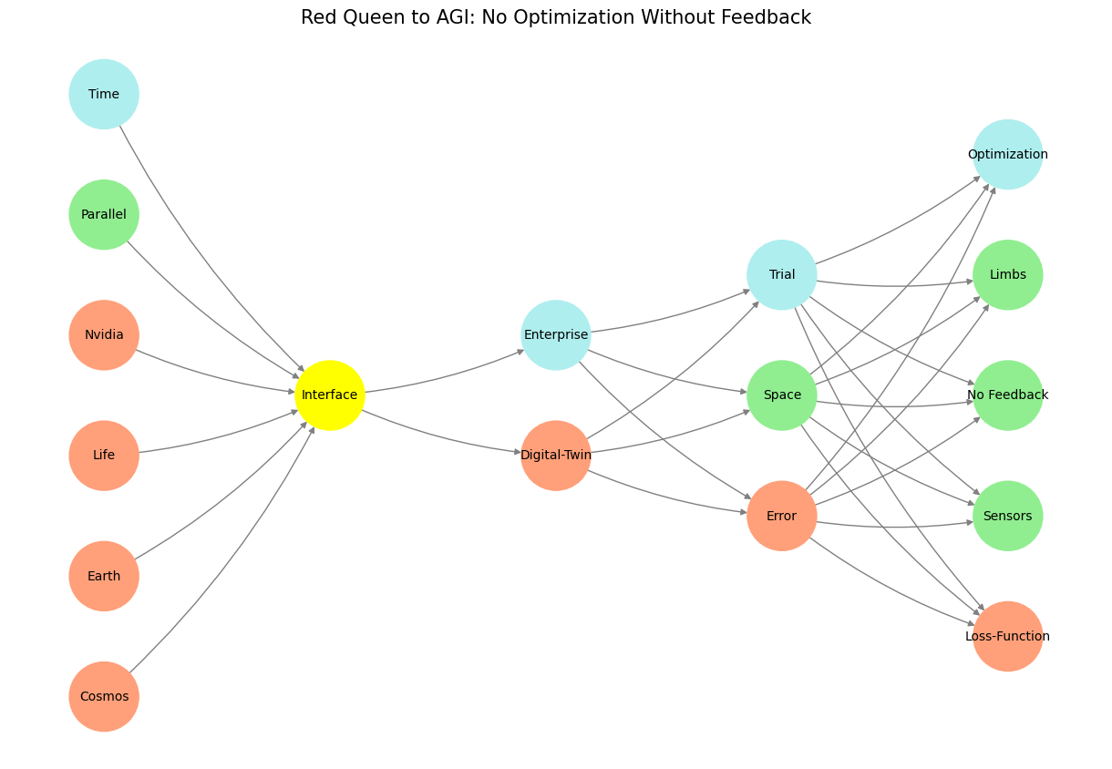
Fig. 4 How now, how now? What say the citizens? Now, by the holy mother of our Lord, The citizens are mum, say not a word.