Life ⚓️

Life ⚓️#

The Strategic Bequest Motive #

B. Douglas Bernheim
Stanford University

Andrei Shleifer
Harvard University

Lawrence H. Summers
Harvard University

Although recent research suggests that intergenerational transfers play an important role in aggregate capital accumulation, our understanding of bequest motives remains incomplete. We develop a simple model of strategic bequests in which a testator influences the decisions of his beneficiaries by holding wealth in bequeathable forms and by conditioning the division of bequests on the beneficiaries’ actions. The model generates falsifiable empirical predictions that are inconsistent with other theories of intergenerational transfers. We present econometric and other evidence that strongly suggests that bequests are often used as compensation for services rendered by beneficiaries.

Tell me, my daughters
(Since now we will divest us both of rule,
Interest of territory, cares of state),
Which of you shall we say doth love us most,
That we our largest bounty may extend
Where nature doth with merit challenge.
[Shakespeare, King Lear]

Fig. 7 Veni-Vidi, Veni-Vidi-Vici. Yep, Red Queen Hypothesis all the way. Off to Mars!#

I. Theoretical Framework#

The notion that rules governing the division of bequests may influence actions taken by potential beneficiaries is not a new one. Indeed, Becker \((1974, 1981)\) has argued that variations in transfers to selfish children force these children to consider their parents’ interests. This is the basis for his rotten kid theorem, which establishes that each beneficiary, no matter how selfish, maximizes the total family income available to the altruistic benefactor. In effect, the benefactor’s welfare is maximized even though he does not design a rule for dividing his estate with the intent of providing incentives for beneficiaries.

In this paper, we advance and test a theory of bequests in which the testator intentionally manipulates the behavior of his beneficiaries through his choice of a rule for dividing his estate. The fundamental difference between Becker’s model and ours is that in our model influence is strategic, while in Becker’s it is nonstrategic. As we shall see, this distinction may be of profound importance in a variety of policy-related contexts.

It may appear that there is no need for a theory of strategic influence: if the rotten kid theorem holds, an altruistic testator cannot improve on the incentives created by automatic (nonstrategic) variations in his bequests. Thus Section IA is devoted to an analysis of the following question: When would a testator wish to improve on these automatic incentives (i.e., behave strategically)? We observe that the validity of Becker’s theorem is limited to cases in which the welfare of testators and beneficiaries alike depends only on monetary income. In particular, if an altruistic testator also cares directly about some action taken by a potential beneficiary (as seems inevitable), nonstrategic incentives will not produce an efficient outcome, let alone maximize the testator’s well-being.

Having established a motive for the exercise of strategic influence on the part of testators, we turn to a second question: When can testators successfully manipulate behavior, and how do they do so? We argue in Section \(1B\) that success in this regard requires the testator to have at least two individuals (or institutions) whom he could credibly name as beneficiaries. When this condition is satisfied, testators can design a rule for dividing bequests that extracts the full surplus generated from interactions with beneficiaries. Otherwise the testator cannot successfully precommit himself to any scheme that improves on automatic incentives.

A. Altruism and Strategic Interaction#

We begin with a brief exposition of the rotten kid theorem. Suppose there are two agents, a parent \((p)\) and a child \((k)\). The child is selfish in the sense that his utility is a function only of his own consumption, \(c_k\). The parent, on the other hand, is altruistic in the sense that he cares both about his own consumption, \(c_p\), and about his child’s utility. We write these utility functions as \(U_k(c_k)\) and \(U_p[c_p, U_k(c_k)]\), respectively.

Suppose that agent \(i (i = k, p)\) has income \(y_i\). Suppose also that the child takes some action that affects both \(y_k\) and \(y_p\); subsequent to this choice, \(p\) makes a utility-maximizing transfer to \(k\). The rotten kid theorem states that \(k\) will choose an action that maximizes total family income, \(y = y_k + y_p\) (and therefore that maximizes the parent’s welfare).

We illustrate this principle in Figure 1. Let \(y^1\) and \(y^2\) be two distinct levels of family income. Each defines an opportunity set for the parent in terms of achievable levels of \(c_k\) and \(c_p\). As long as the parent is not at a corner (his transfer to the child is positive), the allocation of consumption between \(p\) and \(k\) is determined as the tangency between these budget constraints and the parent’s indifference curves. Thus, assuming \(c_k\) is a normal good for the parent, the child maximizes his own welfare by choosing an action that maximizes \(y\). In this context, the parent has no need to manipulate his child’s decision since automatic adjustments in transfers create optimal incentives. It should also be apparent from Figure 1 that a forced transfer from \(p\) to \(k\) will have no effect on either’s level of consumption as long as the parent is not at a corner. This is the basis of the Ricardian equivalence theorem.

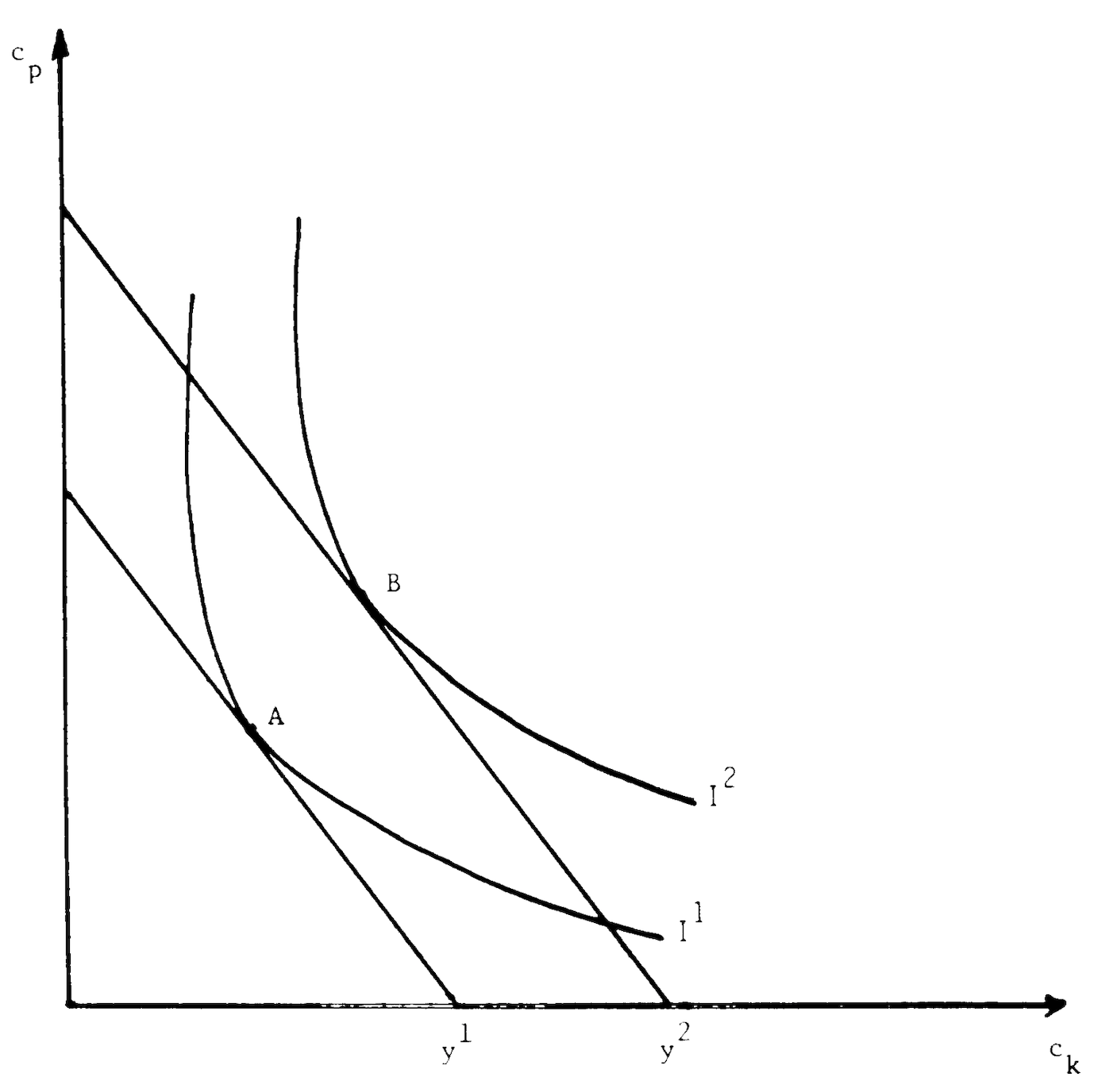
../_images/rotten-kid.png — Fig. 8 An Illustration of the rotten kid theorem#

However, even if testators care about the well-being of their beneficiaries, they may not be perfect altruists. Examples abound: An individual might desire more attention from his own children, object to a relative’s choice of spouse, or want to be cared for by a sibling or grandchild. Institutions (such as universities) commonly treat wealthy patrons particularly well, perhaps to encourage further support in the form of gifts and bequests. In such cases, the rotten kid theorem does not hold.

For concreteness we consider our previous example, modified as follows. First, \(y_p\) and \(y_k\) are fixed. Second, the child takes some action, \(a\), which we will think of as attention given to the parent (visits, care, etc.). Both the parent and the child care about \(a\) directly. Thus, utilities are given by \(U_k(c_k, a)\) and \(U_p[c_p, a, U_k(c_k, a)]\).

We assume that the child’s utility first increases and then decreases in \(a\). The parent’s utility, with \(U_k\) kept constant, always increases in \(a\) initially, though it may decline in \(a\) for high enough attention levels. In fact, we assume something stronger, namely, that parents tire of attention only after children do, if at all (i.e., \(\partial U_p / \partial a > 0\) when \(\partial U_k / \partial a \geqslant 0\)). Finally, in this exposition, we also suppose that the parent’s overall utility (i.e., allowing for the effect of \(a\) on \(U_k\)) declines in \(a\) for high enough \(a\), either because he gets tired of attention or because his concern for his child’s disutility dominates his direct desire for attention.

As before, the parent selects a transfer to the child subsequent to the child’s choice of \(a\). What is the resulting allocation of consumption and attention?

We illustrate the solution to this problem in Figure 2. By substituting for \(c_p (= y - c_k)\) in \(p\)’s utility function, we can represent \(p\)’s preferences entirely in the \((a, c_k)\) plane. Point \(D\) represents \(p\)’s global maximum; \(I_p^1\), \(I_p^2\), and \(I_p^3\) are indifference curves for successively lower levels of utility.

For any level of \(a\), how will \(p\) divide resources between himself and \(k\)? The answer to this question is determined by drawing a vertical line at the relevant value of \(a\) and locating a tangency with one of \(p\)’s indifference curves. This procedure generates an optimal response function for \(p\), \(c_k^*(a)\). One cannot say, a priori, whether this curve slopes upward or downward. If the level of \(a\) does not affect \(p\)’s marginal rate of substitution between \(c_k\) and \(c_p\), \(c_k^*(a)\) will be constant, at some level \(c_k^*\), as shown3. In this special case, automatic variations in transfers provide absolutely no incentives for the child!

Anticipating the parent’s response (or lack thereof), the child effectively chooses a point on \(c_k^*(a)\). We therefore superimpose the child’s indifference curves on the diagram (\(I_k^1\), \(I_k^2\)) and look for a tangency with \(c_k^*(a)\). This is given by point \(A\).

../_images/strategic-bequest.png — Fig. 9 An Illustration of the strategic bequest motive#

Where does \(A\) lie relative to \(D\)? Consider a small horizontal movement to the right from \(A\) along \(c_k^*(a)\). By definition, this does not affect \(k\)’s utility; \(c_p\) is unaffected, and \(a\) increases. Since the parent still wants some more attention for his own pleasure, this movement strictly increases his utility. Thus, \(D\) must lie to the right of \(A\), as shown. Put another way, if \(D\) were to the left of \(A\), then a slight increase in \(a\) would be resisted by the parent but would not matter to the child: a possibility we do not admit.

This argument can be made more formally. Consider the derivative

\[ \frac{d U_p}{d a} = \frac{\partial U_p}{\partial a} + \frac{\partial U_p}{\partial U_k} \left( \frac{\partial U_k}{\partial a} + \frac{\partial U_k}{\partial c_k} \frac{\partial c_k}{\partial a} \right) + \frac{\partial U_p}{\partial c_p} \frac{\partial c_p}{\partial a}; \]

\(\partial U_k / \partial a = 0\) since the child is at his optimum; \(\partial c_k / \partial a = 0\) since we are on the parent’s optimal response schedule; and \(\partial c_p / \partial a = 0\) since that schedule is horizontal. Hence if \(\partial U_p / \partial a > 0\) (and we assume that it is when \(\partial U_k / \partial a = 0\)), then \(d U_p / d a > 0\).

Note further that since \(A\) lies on \(c_k^*(a)\), \(p\)’s indifference curve through this point (\(I_p^1\)) must be vertical. Since \(k\)’s indifference curve through \(A\) is horizontal, we know that Pareto improvements are possible. In particular, the shaded lens in Figure 2 represents the set of Pareto improvements (\(B\) is \(p\)’s most preferred point in the set). Note that all Pareto-improving points involve a larger transfer and more attention than does the autarkic point \(A\).

We summarize these results as follows: Suppose that an altruistic parent cares directly about the level of attention supplied by his child. Suppose also that the level of attention chosen does not affect the parent’s marginal rate of substitution between his child’s consumption and his own consumption. Finally, suppose the parent would, as a direct effect, prefer more attention whenever the child wants to supply more attention. Then, regardless of how much the child likes to supply attention, the level of attention induced by automatic incentives is less than the parent’s global optimum. Furthermore, Pareto improvements are available, all of which entail more attention and a larger transfer to the child.

Under these circumstances the parent will not want to respond passively to the child’s choice. If possible, he will precommit himself to something other than the automatic incentive scheme. Suppose, for the moment, that a threat to disinherit the child, leaving him with consumption, \(c_k^0\), is credible. What should the parent do? Once again refer to Figure 2. If disinherited, the child would pick point \(E\). For his threat to be effective, the parent must insist on an action that leaves the child at least as well off as he was at \(E\). Point \(C\) satisfies this condition and yields the parent more utility than any other such point. Thus the parent would offer the child point \(C\), with the threat of disinheritance if the child refuses. In Section \(IB\) we will discuss the credibility of such a threat.

So far we have considered only the case where \(c_k^*(a)\) is flat; as mentioned, it may slope upward or downward. If it slopes downward, our summarized results still hold. If it slopes upward, \(A\) may lie to the right of \(D[^4]\). However, except by accident, \(A\) and \(D\) would not coincide. Thus, there is almost always a potential for Pareto improvements and an incentive to engage in strategic manipulation.

In our environment it is easily possible for the Ricardian equivalence theorem to fail even while parents are making altruistically motivated bequests to their children. This will occur as long as children do not prefer their parents’ bliss point to being disinherited, so that marginal increases in parental wealth are used to extract extra attention from children5. To illustrate these assertions, return once again to Figure 2. Redistributions between parent and child simply shift the level of \(c_k^0\). Thus, if parents rely on the automatic incentive scheme \(c_k^*(a)\) (as in Becker’s model) and if corner constraints do not come into play, such transfers will plainly have no real effects. However, in our model, reducing \(c_k^0\) (perhaps through social security or debt) changes the parent’s effective threat (point \(E\)) and therefore alters the solution (point \(C\)). On the margin, bequests are used to “purchase” a commodity from the child. Thus a transfer from child to parent will have a pure income effect, and the fraction returned to the child will depend on the parent’s marginal propensity to consume attention out of lifetime wealth. Since most parents will devote only a very small fraction of lifetime resources to the purchase of attention from children, it is reasonable to expect that this income effect will be small.

B. Strategic Bequests#

We observe both formal and informal means by which a benefactor might commit himself to particular rules regarding the distribution of gifts and bequests. At one extreme he could write and make public an explicit will. At the other extreme he could make informal promises and rely on his reputation for keeping such promises. Yet in each case it is possible for him to renege on his commitment: he might rewrite his will without publicizing this fact, or he might break his promise after the beneficiary has acted as desired. If it were, in fact, optimal for him to do this ex post, he would be unable to improve on automatic incentives since rational beneficiaries would anticipate his defection.

Defection may, however, entail substantial costs: the benefactor may incur legal fees or injure his reputation. If benefits from defection do not exceed these costs, then he can successfully precommit to a strategic incentive scheme.

When is this condition likely to be satisfied? Presumably it is quite unlikely that a benefactor can credibly name any arbitrary individual as a potential recipient of substantial transfers: the costs of defection may be low (he does not care what this individual thinks of him) and the benefits high (he greatly prefers to leave his money to someone else). However, if he is relatively indifferent about the distribution of transfers between certain individuals, he may have substantial scope for precommitment.

Consider two hypothetical examples. First, suppose a parent has a single child, whom he loves far more than anyone else. He wishes to influence this child’s behavior by threatening disinheritance. For this threat to be credible, he must specify an alternative distribution of his estate. Suppose he directs that his entire estate is to be left to some randomly selected third party unless the child complies (perhaps he simply promises the estate to the third party under the relevant contingency). The parent has an enormous incentive to renege on this directive, and the costs of doing so may be quite low (he breaks a promise to a stranger or incurs minimal legal costs)6. If so, the threat is empty.

On the other hand, suppose the parent has two children, both of whom he loves more than anyone else. Again he wishes to influence the behavior of one child by threatening disinheritance. Suppose he directs that his entire estate is to be left to the other child unless the first child complies. His incentive to renege on this directive is far less than in the first case (he loves both children). His costs may also be small since he may be more hesitant to break a promise to one of his children7. Thus the threat may well be credible.

To summarize: The costs and benefits of defection determine a set of distribution rules to which the benefactor can successfully commit himself (he lacks sufficient incentive to defect). Presumably, each of these rules has the property that virtually all transfers are made to individuals (or institutions) about whom the benefactor cares very much. Regarding transfers to these individuals (whom we shall hereafter call “credible beneficiaries”), the benefactor may have substantial scope for precommitment. Indeed, it may be credible for him to specify any distribution of transfers as long as everything is distributed within this group.

The identification of the credible beneficiaries for any particular benefactor is an empirical issue. This set may be limited to children or may include other relatives, friends, employees, or institutions. Factors other than personal preference may also come into play: in some states, courts protect children’s claims on their parents’ estates. For the time being we will merely assume that this set is identifiable but will avoid identifying it. For simplicity we will also assume that it is credible to specify any distribution of transfers within this group (the analysis changes very little if the set of credible distribution rules is further constrained).

Formally, we modify the framework adopted in Section IA as follows. First, we introduce additional potential beneficiaries. Second, we assume that the benefactor can commit himself in advance both to the total size of his bequest (perhaps by holding wealth in illiquid forms, such as durables and housing) and to a rule governing the division of this bequest.

In particular, we assume that the utility of the benefactor is given by \(U_p(c_p, a_1, \ldots, a_N, U_1, \ldots, U_N)\), where \(a_n\) is some action taken by the \(n\)th potential beneficiary and \(U_n\) is the utility of this beneficiary. Further, \(U_n\) is given as some function of \(a_n\) and \(c_n\) (\(n\)’s consumption), \(U_n(c_n, a_n)\). For notational convenience we define \(a = (a_1, \ldots, a_N)\). The benefactor makes a transfer, \(b_n\), to each beneficiary. He is constrained to choose

\[ b_n \geqslant 0, \]

\[ c_p + \sum_{n=1}^N b_n \leqslant y_p . \]

The consumption of each beneficiary is then given by \(c_n = c_n^0 + b_n\).

Formally, the game proceeds as follows. First, the benefactor locks in his total bequest (thereby determining his own consumption as a residual) and commits himself to a “bequest rule,” which governs the division of his estate. This rule specifies, for each profile of actions \(a\), that a fraction \(\beta_n\) of total bequest be given to each beneficiary \(n\). We represent this rule as a profile of \(N\) functions:

\[ \beta^*(a) = [\beta_1^*(a), \ldots, \beta_N^*(a)] . \]

We require that the bequest rule satisfy only one condition: for all \(a\), \(\sum_{n=1}^N \beta_n^*(a) = 1\). This restriction reflects two considerations. First, for feasibility, the sum of shares cannot exceed unity. Second, the benefactor must bequeath anything that he does not consume (in this model, he lives for only one period), and, by assumption, he cannot bequeath anything to anyone other than his credible beneficiaries.

After the benefactor has made these choices, potential beneficiaries select levels of \(a_n\). Finally, the estate is divided according to the specifications of the bequest rule. Note that we could consider a multiperiod version of this model, which has an additional implication that parents hold wealth in both bequeathable and annuitized forms. Such an extension is presented in Bernheim, Shleifer, and Summers (1984) and produces the same conclusions as the model we analyze here.

We motivate the solution to this game as follows. Consider the set

\[ S_n = \{(a_n, b_n) \mid U_n(c_n^0 + b_n, a_n) \geqslant U_n(c_n^0, a_n^0)\}, \]

where \(a_n^0\) is the level of \(a_n\) that \(n\) would choose in the absence of transfers. Graphically, \(S_n\) corresponds to the set of points above (and including) the indifference curve \(I_k^2\) in Figure 2. Since each beneficiary receives a nonstrategic transfer, he can, at worst, be disinherited. Thus, any equilibrium must involve beneficiary \(n\)’s consuming an allocation in \(S_n\).

Now consider the following artificial problem for the benefactor:

\[ \max_{a, \beta, c_p} U(c_p, a, U_1, \ldots, U_N) \]

subject to

\[ U_n = U_n[a_n, c_n^0 + \beta_n(y_p - c_p)], \]

\[ [a_n, c_n^0 + \beta_n(y_p - c_p)] \in S_n . \]

The solution to this problem, denoted \((a^*, \beta^*, c_p^*)\), would be appropriate if the benefactor could choose actions for potential beneficiaries subject only to the constraint that each is willing to participate. Now assume that there is a bequest rule, \(\beta^\circ\), that, along with \(c_p^*\), induces \(a^*\) as equilibrium choices for the beneficiaries and satisfies \(\beta^\circ(a^*) = \beta^*\). Since the resulting allocation achieves an optimum ignoring incentive constraints, it must necessarily be the benefactor’s best choice when these constraints are imposed. In equilibrium, play would then evolve as follows: the benefactor would choose \(c_p^*\) and \(\beta^\circ\), the beneficiaries would play \(a^*\), and the estate would be divided accordingly (\(n\)’s share would be \(\beta_n^*\)).

To characterize equilibrium for this game, we need only exhibit a bequest rule, \(\beta^\circ\), for which \(a^*\) emerges as an equilibrium in the beneficiaries’ subgame (when \(c_p = c_p^*\)), and \(\beta^\circ(a^*) = \beta^*\). One such rule operates as follows. We will refer to \(a_n^*\) as \(n\)’s “benchmark” action. Denote the set of beneficiaries who take at least their benchmark actions by \(B = \{n: a_n \geqslant a_n^*\}\). Let \(\bar{B}\) denote the complement of \(B\). If \(B\) is nonempty, the benefactor bequeaths nothing to members of \(\bar{B}\). In contrast, if \(n\) is a member of \(B\), then \(n\)’s share will be

\[ \beta_n = \frac{\beta_n^*}{\sum_{j \in B} \beta_j^*} . \]

If \(B\) is empty, then the benefactor bequeaths everything to the beneficiary, \(m\), whose action is closest to his benchmark level: \(a_m^* - a_m \leqslant a_n^* - a_n\) for all \(n\). This bequest rule is intuitively appealing: each beneficiary normally receives a positive bequest but is disinherited if he fails to meet a standard of “good” behavior. If all children are “bad,” the “best” child receives the entire estate.

This rule defines a simultaneous move subgame where potential beneficiaries choose actions \(a_k\). It is easy to verify that there are \(N + 1\) Nash equilibria for this subgame; one consists of every beneficiary playing his benchmark level. In the remaining \(N\) equilibria, \(N - 1\) beneficiaries choose their benchmark levels, while the last one (l) chooses \(a_l\). However, for a variety of reasons one can safely ignore these less desirable equilibria8.

Note that this construction depends integrally on the assumption that \(N \geqslant 2\). If \(N = 1\), then \(\beta_1 = 1\) for all admissible bequest rules. The sole potential beneficiary knows that his behavior cannot affect his inheritance; thus the benefactor is unable to influence his behavior.

Stepping outside of our formal structure, one might imagine other means by which a benefactor could motivate a sole beneficiary. For example, he might precommit to some rule that conditioned his own consumption on the beneficiary’s action. This is, however, far more difficult than “locking in” a fixed total bequest (by holding wealth in illiquid forms) as in our model. First, he cannot credibly commit to giving the beneficiary less than his automatic bequest, \(c_k^*(a)\); to renege, he need only break a promise to himself (this involves neither legal costs nor a damaged reputation). Thus, his scope for manipulation is severely limited. Second, he may have large incentives to renege on the promise of rewards above this automatic level since the level of his own consumption is at issue (he cannot lock in these incremental rewards in advance, or they would have no influence on the beneficiary’s choice).

To summarize: When a benefactor can successfully threaten to disinherit a potential beneficiary, he extracts the full surplus generated through interaction with the beneficiary. However, success in this regard requires him to specify an alternative use for his resources that is believable; in particular, he must have more than one potential beneficiary to whom he can credibly plan to leave the bulk of his estate.

The analysis presented in Sections \(1A\) and \(1B\) suggests several possible ways of distinguishing between this theory and its competitors. First, evidence that the behavior of children is influenced by anticipated bequests would support the class of models in which bequests function as a medium of exchange. Second, evidence suggesting that parents successfully wield influence only when they have more than one credible beneficiary would support the particular theory of strategic influence outlined above. Third, evidence suggesting that parents care directly about some actions taken by their children would establish the motive for strategic as opposed to nonstrategic influence (as in Becker’s rotten kid theorem).

II. Econometric Evidence#

In this section we provide empirical support for the hypothesis that bequests are used, in part, to influence the behavior of potential beneficiaries. Specifically, our examination of microeconomic panel data reveals that contact between parents and children is much higher in families where the elderly parent has a substantial amount of bequeathable wealth to offer. We show that this correlation is robust with respect to a variety of specifications and estimation techniques, which are designed to rule out alternative explanations based on potentially spurious factors. In addition, we explore some implications of the particular model developed in Section I that differentiate it from closely related alternatives and use these implications to test the model. The results are extremely favorable to our formulation of strategic bequests.

Bequests can serve as a means of payment for services only if the presence of bequeathable wealth can influence the behavior of potential beneficiaries and if testators exercise this influence. We adopt a slight abuse of terminology, referring to these two distinct aspects of exchange as the “supply” and “demand” sides. Primarily because of the nature of available data, our basic strategy is to estimate the effect of bequeathable wealth on the amount of services beneficiaries provide to testators—the supply side. Although we do not estimate the demand side explicitly, we provide indirect statistical evidence for the claim that testators exploit the relationship between services and bequests.

The econometric investigation detailed below requires rather specific data concerning assets and family interactions for a sample of elderly individuals. The Longitudinal Retirement History Survey (LRHS), conducted by the Office of Research and Statistics of the Social Security Administration, collected surprisingly extensive information on these characteristics. Data from the 1969, 1971, 1973, and 1975 waves of the LRHS were available at the time of this writing; unfortunately, insufficient data on assets were collected in 1973, so we were forced to drop this year. Over 11,000 individuals aged 58-63 were included in the first wave. Many of these were lost to attrition; on top of this we restricted our sample to married couples who had at least one child but no children living at home and for whom sufficient data on nonbequeathable assets were available9. Our final sample consisted of 1,166 observations, 855 of which had two or more living children and 311 of which had only one living child.

Measures of contact between parents and children were constructed as follows. For each observation the LRHS contains information on total number of children (\(C_i\)), number of children who visit or telephone their parents weekly (\(VW_i\)), and number of children who visit or telephone their parents monthly (\(VM_i\))10. Our measure of attention per child was constructed from these variables as follows:

\[ V_i = \frac{4 \cdot VW_i + VM_i}{4 \cdot C_i}, \]

where \(V_i\) indicates contact per child, normalized so that maximum contact equals unity. We have adopted the approximation that children who visit weekly give their parents four times as much attention as those who visit monthly. It is interesting to note in passing that the mean of \(V_i\) was 0.54 in 1969 and rose to 0.63 in 1975—evidently the average level of contact is quite high and rises with age.

Other variables were constructed as follows. Bequeathable wealth per child (\(b_i\)) includes financial wealth (stocks, bonds, mutual funds, bank accounts, checking accounts), residential and other property, the face value of life insurance11, privately purchased annuities12, and debt. Nonbequeathable annuity wealth per child (\(aw_i\)) includes social security and pension wealth. These were obtained by converting data on income from those sources to capitalized values applying a discount rate of 1.03 and actuarial survival probabilities. Matching administrative records contained data on income earned from 1951 to 1975 in employment covered by social security up to the taxable maximum. This information was extrapolated to yearly earnings using the method described in Fox (1976). The resulting income stream was then accumulated at a 3 percent rate of return to produce a measure of lifetime earnings for both husband and wife. Other variables used in the following analysis included age of respondent and dummy variables indicating whether the respondent’s health is better (\(BH_i\)) or worse (\(WH_i\)) than that of other members of his cohort, as well as whether the respondent is retired (\(RET_i\)).

One practical difficulty with these data is that information on the behavior of potential beneficiaries is limited to children. For any given individual the set of credible beneficiaries may or may not be larger. Since our theory suggests that successful exchange takes place only when this set contains at least two candidates, we cannot be certain that single-child families will behave in the manner predicted here. Consequently, we initially restrict attention to families with two or more children. Analysis and discussion of behavior in single-child families are deferred to the end of this section.

Another general issue that arises with regard to the use of these data concerns the treatment of separate sample years. Except where noted, results presented in this paper are based on simple pooling of the sample years. No correction is made for potential correlation between distinct observations on the same household. Such correlation would not, by itself, cause our estimates to be inconsistent; however, it would imply that standard errors are calculated incorrectly. In order to determine the probable magnitude of the resulting error, we reestimated a number of our specifications employing the appropriate generalized least squares (GLS) correction. Although small changes in some point estimates were noted, no qualitative conclusions were altered. More important, estimated standard errors on critical coefficients (such as \(b_i\)) differed only slightly from those obtained with simple pooling.

We begin our analysis by specifying the supply of attention from children as a function of potential bequest per child:

\[ V_i = \beta_0 + \beta_1 b_i + \epsilon_i \]

where \(V_i\) and \(b_i\) are defined above and \(\epsilon_i\) is a random error term. Within the context of our theoretical model, one can think of equation (2) as a linear approximation to the implicit function defined by (1), aggregated over beneficiaries.

Our first step was to estimate equation (2) using ordinary least squares (OLS)13. Results are presented as equation (i) in Table 1. While the sign of the coefficient on \(b_i\) is consistent with our theory, one cannot reject the hypothesis that bequeathable wealth holdings have no effect on attention per child.

There are, however, a variety of reasons for believing that OLS estimates of this relationship may be inconsistent. One reason follows directly from the structure of our model: explicit consideration of the demand side suggests that \(b_i\) will be determined endogenously. The parent’s optimal choice of \(b_i\) depends in part on the preferences of his children, and \(\epsilon_i\) is an important component of these preferences. Thus, as long as the parent has more information about the preferences of his children than does the econometrician, \(b_i\) and \(\epsilon_i\) will be correlated. The direction of the resulting bias is, however, ambiguous.

Correlation between \(b_i\) and \(\epsilon_i\) is likely to be present for other reasons as well. Stepping outside the formal model of the last section, one particularly plausible story is that some parents get along well with their children while others do not. Those that do may hold more bequeathable wealth simply because they like their children, while the children in turn may be attentive simply because they like their parents.

Our solution to this set of problems is to instrument for \(b_i\) in equation (2) using the parents’ lifetime earnings \(y_i\). We justify this choice of instrument as follows. It is clear that lifetime earnings are positively correlated with holdings of bequeathable wealth. We must establish that, in addition, this instrument is uncorrelated with \(\epsilon_i\). For our first story, \(y_i\) may be correlated with \(\epsilon_i\) if parents work harder when young, so that they have more wealth with which to influence their children when old. For our second story, this correlation may be nonzero if the elderly parents whose children particularly like them have been particularly hardworking (or lazy)14. Although one could, in both cases, plausibly argue that the correlation is nonzero, it is difficult to believe that it is very large.

Two-stage least squares (2SLS) estimates of equation (2) are presented as equation (ii) of Table 1. Notice that the coefficient on \(b_i\) is approximately eight times as large as the corresponding OLS estimate and that the hypothesis of no effect on attention can be rejected at extremely high levels of confidence. This regression confirms our prediction that, in multiple-child families, bequeathable wealth will be strongly correlated with attention.

The apparently striking difference between OLS and 2SLS estimates can be tested formally. A Hausman (1978) test reveals that exogeneity of \(b_i\) can be rejected at a high level of confidence. This conclusion is consistent with our model (in which \(b_i\) and \(a_i\) are simultaneously determined) and constitutes limited evidence in favor of an operative demand side. One should, of course, bear in mind that this rejection of exogeneity is also consistent with other alternatives. Nevertheless, it is worth noting that the particular alternative outlined above (correlation between filial and parental altruism) implies that OLS estimates of the coefficient on \(b_i\) should be biased upward. In fact, we observe the opposite.

While our theoretical model offers one explanation for the set of results described above, the observed correlation between attention and bequeathable wealth could also be attributed to a number of spurious factors. We now turn to the task of ruling out these alternative explanations.

One might object that our basic specification omits a number of important variables with which both attention and bequeathable wealth are highly correlated. For example, healthy parents may be more pleasant to visit (or, conversely, less needy of attention) as well as more successful in the marketplace. Older parents belong to a poorer cohort and in general require more care. Retired parents may have a greater desire for contact with children. We correct for these difficulties by adding a vector of parental characteristics, \(\mathbf{Z}_i\), to our basic specification:

\[ V_i = \beta_0 + \beta_1 b_i + \mathbf{Z}_i \gamma + \epsilon_i \]

In particular, \(\mathbf{Z}_i\) includes age, health dummies (\(BH_i\), \(WH_i\)), and a retirement dummy (\(RET_i\)). Results are presented as equation (iii) in Table 1. The inclusion of these additional variables appears to have very little impact on either the magnitude or statistical significance of the coefficient on \(b_i\).

Another apparently compelling objection is that wealth may affect attention through a variety of spurious channels. For example, parents with higher wealth may simply pay for traveling expenses, telephone calls, and so forth in order to have more contact with their children. Wealth effects may also be less direct. In particular, there is presumably a positive correlation between the incomes of parents and those of their children. A wealthy child may be more difficult to influence or more desirable to visit. Wealthy children may be more capable of defraying the costs of travel and telephones but may also, on average, live farther from their parents. Thus the direction of the potential bias is not obvious.

Note, however, that these alternative explanations do not distinguish between bequeathable and nonbequeathable wealth (social security and pension annuity), as does our theory. A parent’s ability to defray the costs of contact is determined both by his ordinary wealth and by his claims on annuities. Similarly, while it is true that the wealth of children is correlated with parental resources, it is not likely to be highly correlated with the division of parental resources between bequeathable and nonbequeathable forms. Thus, in order to determine the magnitude of spurious wealth effects, we add annuity wealth (\(aw_i\)) to our basic specification:

\[ V_i = \beta_0 + \beta_1 b_i + \beta_2 aw_i + \mathbf{Z}_i \gamma + \epsilon_i . \]

The effect of holding another dollar of wealth in bequeathable form is then given by the difference between the coefficients on \(b_i\) and \(aw_i\) (\(\beta_1 - \beta_2\))15.

Estimates of specification (4) are presented as equation (iv) in Table 1. Note that the coefficient on \(aw_i\) (the spurious wealth effect) is negative and statistically significant, while the coefficient on \(b_i\) is positive and highly significant. The effect of holding wealth in bequeathable rather than annuitized form, given by the difference between these coefficients, is estimated to be 6.36, with a standard error of 1.89. Thus, correcting for spurious wealth effects only strengthens our original conclusion.

Another possible solution to the problem of spurious wealth effects is to restrict attention to a subsample for which these effects are likely to be unimportant. If the source of contamination concerns ability to pay, then such effects may be minimized by considering a subsample for which financial costs of contact are negligible. Presumably, geographic proximity eliminates much of these costs. Fortunately, the LRHS contains relevant information. Accordingly, we reestimated equation (4) for two subgroups: parents whose children all live within the same city or neighborhood and parents whose children all live within 150 miles. The parameter estimates (omitted)16 were quite close to those obtained for the entire sample. In fact, the effect of bequeathable wealth on attention appeared to be largest for parents living in closest proximity to their children.

A related objection concerns the inclusion of housing wealth in our measure of \(b_i\). It has been suggested to us that a positive coefficient on \(b_i\) may simply reflect the fact that children prefer to visit parents who live in nice houses. To accommodate this objection, we reestimated equation (4), substituting bequeathable nonhousing wealth (\(bnh_i\)) for \(b_i\). Despite the fact that most elderly individuals hold a large fraction of their portfolios in residential housing, the estimates (omitted) were very close to those presented in Table 1; in fact, the estimated bequeathable wealth effect was slightly larger. On the basis of this evidence, we are inclined to reject the hypothesis that our results are simply an artifact of some special feature of housing wealth.

As a final check on the robustness of our results, we reestimated equation (4) separately for each of our sample years. The coefficients of interest (those on \(b_i\) and \(aw_i\)) were extremely stable over the sample period (estimates are omitted).

So far, our empirical analysis has been solely concerned with establishing a link between attention and bequeathable wealth and with ruling out alternative explanations based on potentially spurious factors. We now explore some other implications of the particular model developed in Section I that differentiate it from closely related alternatives, and we use these implications to test the model.

First, a number of the variables included in \(\mathbf{Z}_i\) should affect the “price” at which attention can be purchased, as well as the absolute amount of attention supplied by children. Consider, for example, the variable \(WH_i\) (worse health). Although sick parents may receive more attention simply because of filial devotion, in a more cynical view, illness increases the probability of death, thereby making a potential bequest of fixed magnitude more valuable to the child. To differentiate between these effects, we reestimated equation (4), adding interactions between \(b_i\) and \(WH_i\), \(BH_i\), and \(AGE_i\)17. The results, presented as equation (v) of Table 1, are quite striking. Only three coefficients are statistically significant: those on \(aw_i\), \(WH_i\), and \(WH_i \cdot b_i\). The coefficient on \(aw_i\) changes very little from our original estimate. The coefficient on \(WH_i\) is negative, indicating that, aside from exchange-motivated concerns, sick parents receive less attention. In contrast, the coefficient on \(WH_i \cdot b_i\) is large and positive. This strongly suggests that, for multiple-child families, rich parents (where “rich” is strictly defined in terms of bequeathable assets rather than total resources) who are in poor health receive much more attention than their indigent counterparts. Once again, the data suggest significant financial motivation.

A second strong implication of our particular theory is that exchange-motivated holding of bequeathable wealth can influence the behavior of potential beneficiaries only if there are at least two credible candidates. Unfortunately, as mentioned above, there is no way to determine the number of such candidates for any particular respondent in the LRHS. However, logically speaking, our theory admits the possibility that children are, in some meaningful sense, the only credible beneficiaries for the bulk of a parent’s estate. This hypothesis can be tested empirically by investigating behavior in single-child families and comparing it with our multiple-child results. We must emphasize that this hypothesis is not a consequence of our theory; thus failure to differentiate between behavior in single- and multiple-child families would not recommend rejection of our theory. However, the absence of a positive correlation between attention and bequeathable wealth in single-child families would strongly support our theory, as well as the supplemental hypothesis that parents cannot credibly threaten to disinherit all of their children.

These considerations motivated us to reestimate each specification above using data on single-child families. Our results are presented in Table 2. Note that in equations (i)-(iv) the pattern of signs on the coefficients on \(b_i\) and \(aw_i\) is precisely the opposite of that obtained for multiple-child families. In addition, the standard errors of coefficients on key parameters are relatively small. It is worth noting that the coefficient on \(b_i\) in these regressions is quite close to the magnitude of the spurious wealth effect estimated for multiple-child families18. This is what one would expect, since \(b_i\) is no longer “contaminated” by strategic considerations. The only troubling aspect of these estimates is that there appears to be a statistically significant difference between the coefficients on \(b_i\) and \(aw_i\); presumably, \(aw_i\) should carry only the spurious wealth effect as well. Strictly speaking, this is inconsistent with our model. Note finally that in equation (v), worse health continues to have a negative impact on attention (although the magnitude is not statistically significant); however, there is no evidence that this can be compensated for by high bequeathable wealth holdings, as in multiple-child families. This evidence strongly supports the hypothesis that strategic bequests take place only in families with at least two children; thus children are usually the only credible beneficiaries. It is difficult to reconcile this conclusion with any known model of bequests other than that presented in Section I.

One possible explanation for our findings is that the results on the multiple-child family are an artifact caused by estimating across families of different sizes. As a check against this possibility, we reestimated equation (4) separately for two- and three-child families. Results are presented in Table 3. For both groups, key parameter estimates are very close to those obtained for the original sample19.

A further remark on the difference between single- and multiple-child families is in order. Just as it is difficult to see how this difference could be reconciled with any other known theory of bequests, it is also difficult to see why any explanation of our multiple-child results based on potentially spurious factors would not apply equally well to single-child families. Thus, our results refute any alternative explanation that fails to account for the single/multiple child distinction. We believe that this makes the empirical case for our theory compelling.

Taken as a whole, the preceding estimates are extremely favorable to our model. It is therefore important to emphasize that our results are extremely robust and that these estimates are representative of other regressions we ran but did not include in this paper. Aside from some problems with selecting a proper subsample (e.g., one preliminary sample inadvertently included observations of which children lived at home, making interpretation of visits and telephone calls difficult), our procedures produced favorable results on the first try, and subsequent modifications did not alter any substantive conclusions. Full disclosure requires that we report three apparent “failures.” First, OLS estimates of all but the simplest specification (eq. [i], Table 1) yielded negative coefficients on \(b_i\). This is not surprising in the light of our arguments concerning the endogeneity of \(b_i\); in fact, we submit that the discrepancy between OLS and 2SLS estimates strengthens the case for an operative demand side. Second, attempts to estimate a fixed-effects version of the model produced nonsensical coefficients with large standard errors. However, since no sensible instrument is available for fixed-effects estimation (there is only one observation on lifetime earnings for each respondent), we were not troubled by this finding. Finally, estimates based on an alternative measure of attention (letters received from children) were much less striking. Although the pattern of coefficients was consistent with our theory (the coefficient on \(b_i\) was greater than the coefficient on \(aw_i\) for multiple-child families, and vice versa for single-child families), alternative hypotheses could not be rejected with any reasonable level of confidence. On reflection we decided that the letters variable was not a very satisfactory proxy for attention since parents who were frequently visited presumably received few letters.

Table 1#

	OLS (Eq. [i])	2SLS (Eq. [ii])	2SLS (Eq. [iii])	2SLS (Eq. [iv])	2SLS (Eq. [v])
Constant	.560 (.008)	.531 (.013)	.088 (.201)	.225 (.215)	.230 (.350)
\(b \cdot 10^6\)	.333 (.308)	2.30 (.686)	2.57 (.715)	4.58 (1.18)	8.51 (18.4)
\(aw \cdot 10^6\)	…	…	…	-1.78 (.820)	-1.85 (.867)
\(AGE / 100\)	…	…	.722 (.311)	.513 (.332)	.529 (.549)
\(BH / 100\)	…	…	-2.55 (1.79)	-2.96 (1.84)	-2.41 (4.21)
\(WH / 100\)	…	…	-1.37 (2.43)	-2.984 (2.49)	-24.2 (8.22)
\(RET / 100\)	…	…	-2.22 (1.89)	-3.26 (1.99)	-3.67 (2.03)
\(b \cdot AGE / 10^7\)	…	…	…	…	-.756 (2.92)
\(b \cdot BH / 10^7\)	…	…	…	…	-.731 (20.7)
\(b \cdot WH / 10^7\)	…	…	…	…	237 (80.3)
Degrees of freedom	2,563	2,563	2,559	2,558	2,555
Standard error of regression	.357	.360	.360	.369	.374

Table 2#

Sample: Single-Child Families—Pooled Panel (Dependent Variable \(V\))#

	OLS (Eq. [i])	2SLS (Eq. [ii])	2SLS (Eq. [iii])	2SLS (Eq. [iv])	2SLS (Eq. [v])
Constant	.639 (.018)	.653 (.029)	-.489 (.409)	-.651 (.423)	-.688 (1.05)
\(b \cdot 10^6\)	-.662 (.288)	-1.00 (.615)	-1.23 (.628)	-2.37 (.864)	1.31 (24.7)
\(aw \cdot 10^6\)	…	…	…	1.26 (.618)	.987 (.658)
\(AGE / 100\)	…	…	1.89 (.631)	2.12 (.649)	2.16 (1.65)
\(BH / 100\)	…	…	-3.36 (3.60)	-2.27 (3.69)	5.82 (9.22)
\(WH / 100\)	…	…	-11.8 (5.07)	-11.56 (5.13)	-12.6 (10.1)
\(RET / 100\)	…	…	5.47 (3.86)	-4.83 (3.92)	-5.82 (4.07)
\(b \cdot AGE / 10^7\)	…	…	…	…	-.448 (3.95)
\(b \cdot BH / 10^7\)	…	…	…	…	-18.3 (19.6)
\(b \cdot WH / 10^7\)	…	…	…	…	.251 (24.9)
Degrees of freedom	931	931	927	926	923
Standard error of regression	.451	.451	.446	.452	.453

Table 3#

Sample: Multiple-Child Families—Pooled Panel (Procedure: 2SLS; Dependent Variable \(V\))#

	Two-Child Families (Eq. [iv])	Three-Child Families (Eq. [iv])
Constant	.065 (.350)	-.164 (.370)
\(b \cdot 10^6\)	3.12 (1.31)	3.79 (3.26)
\(aw \cdot 10^6\)	-1.11 (1.06)	-1.45 (1.37)
\(AGE / 100\)	.728 (5.36)	1.24 (.573)
\(BH / 100\)	.929 (2.74)	-9.74 (3.43)
\(WH / 100\)	1.86 (4.24)	-.802 (4.41)
\(RET / 100\)	-.229 (3.15)	-3.41 (3.42)
Degrees of freedom	1,124	710
Standard error of regression	.383	.345

III. Other Evidence#

The preceding econometric analysis of the LRHS data favors the view that strategic exchange plays an important role in bequest behavior. By and large the predictions of our model are confirmed. At least some of these predictions are not implications of alternative models of bequest behavior. Beyond this evidence there are a number of other aspects of individual behavior that are more easily reconciled by our model of strategic bequests than with alternative formulations.

There are at least three alternative formulations to the present model of bequest behavior that have been widely studied. These are the “accidental bequests,” “bequests for their own sake,” and “altruistic bequests” models. The first, recently urged by Davies (1981), suggests that consumers do not have bequest motives and that bequests arise only as a consequence of uncertainty about the date of death in conjunction with annuity market imperfections. A second model, used by Blinder (1974) and many others, assumes that consumers’ lifetime utility depends in part on the size of their bequest. In this view bequests are a form of terminal consumption. A final possibility is the “altruistic” view of bequests put forth by Barro (1974) and Becker \((1974, 1981)\). In this view parents maximize a utility function in which the utility of their children also enters, but they engage in no strategic behavior.

Each of these formulations is inconsistent with the empirical observation that consumers are reluctant to participate in annuity-type arrangements even on quite favorable terms. Moreover, the second and third formulations cannot account for the apparent insignificance of gifts. We first review the available evidence, then indicate why it contradicts the three standard models of bequest behavior, and finally describe why such behavior is consistent with our model.

Privately purchased annuities are a rarity in the American economy. The LRHS revealed that such annuities rarely represented more than a very small fraction of wealth and, in most cases, were not purchased at all. Of course, this may well be so because adverse selection complicates the working of this market20. Perhaps more persuasive evidence comes from the lack of market response to “reverse annuity mortgages.” These instruments allow individuals to annuitize their home equity. Even where they are offered on relatively favorable terms, they do not appear to be well received21. A similar conclusion is suggested by the lack of response to a California state program that allowed property owners to defer property taxes until after their death on a subsidized basis (see Urban Systems Research and Engineering 1983).

Perhaps the strongest evidence of consumer resistance to annuities comes from an examination of the choices made by retirees under the TIAA-CREF program. This group is mainly composed of educators who are presumably better informed than most pension recipients. Retirees are offered several options, including full annuities and “\(n\)-year certain” plans22. A 10-year certain, for example, guarantees that a retiree and his heirs will receive at least 10 years’ worth of benefits, even if the retiree dies sooner23. A 1973 study reported that over 70 percent of beneficiaries chose plans other than those providing full annuity protection. This suggests a desire to make allowances for bequests.

This evidence suggests that there is no strong latent demand on the part of aged Americans for annuity protection, and it is clearly inconsistent with the accidental bequest model. In this view individuals should purchase annuity protection even if it is very unfair actuarially since bequests are not valued at all. In particular, the choice of years certain annuity protection directly contradicts the accidental bequests model.

Less obviously, the reluctance of consumers to take advantage of actuarially fair or subsidized annuities is inconsistent with the bequests for their own sake and altruistic models of bequests. It is well known (see, e.g., Sheshinski and Weiss 1981; Bernheim 1984a) that under such formulations consumers who have access to actuarially fair annuity markets will perfectly insure, financing consumption entirely out of annuity income. An underannuitized individual will finance consumption partly out of bequeathable wealth, while an overannuitized individual will save some fraction of his annuity income, thereby building an estate. Thus if an individual consumes some portion of either the principal or income from his bequeathable wealth, we infer that he is underannuitized and should take advantage of actuarially fair opportunities to purchase annuities.

There are two reasons to believe that individuals hold bequeathable wealth in part to finance their own personal consumption. First, despite the earlier findings of Brittain (1978) and Mirer (1979), more recent studies by Diamond and Hausman (1982), King and Dicks-Mireaux (1982), and Bernheim (1984b) suggest that retirees do dissave from bequeathable wealth. Second, if bequeathable wealth is held only for the purpose of making intergenerational transfers, then these transfers would be made as gifts rather than as bequests at death. Early transfer confers two advantages: it allows beneficiaries to annuitize the optimal fraction of transferred resources immediately, and it may ease liquidity constraints encountered by beneficiaries early in the life cycle24.

To summarize: Behavioral evidence suggests that individuals hold bequeathable wealth in part to finance personal consumption. Under either the bequests for their own sake or altruistic models, this implies that such individuals are underannuitized and should take advantage of actuarially fair opportunities to insure. Yet this prediction is counterfactual.

The reluctance of very wealthy individuals to convert bequests into intra vivos gifts poses a further puzzle for these alternative theories. Despite the existence of significant tax advantages to transferring resources during lifetimes, many wealthy individuals who can anticipate leaving large bequests with virtual certainty do not make significant intra vivos gifts. This observation has disturbed some proponents of dynastic altruism who recognize that an important implication of this model is that families will conduct their affairs to minimize total tax liability. While some (notably Adams 1978) have defended dynastic altruism by arguing that, contrary to Shoup (1966), Cooper (1979), and Menchik (1980), tax-minimizing transfers are in fact observed, we find this claim implausible25.

The strategic bequest model described in Section I does not share these counterfactual implications concerning the acceptance of annuities and the use of gifts. By making all intentional transfers at once, the parent attenuates his ability to influence his children in subsequent periods (King Lear’s well-known blunder). Furthermore, it is quite likely that it is easier to influence children by promising bequests as opposed to gifts. Few families are so mercenary as to countenance explicit quid pro quo contracts; thus the lure of gifts tends to be more speculative than a claim on a known estate, and vague promises of contemporaneous rewards are subject to equivocation by parents who would prefer to retain resources ex post.

A common finding in empirical analyses of bequests (Sussman et al. 1970; Brittain 1978; Menchik 1980)26 is that, in most cases, parents give equal amounts to each of their offspring. In part, this conclusion may arise from focusing primarily on cash rather than on the more difficult-to-value tangible bequests. The model here makes no prediction that bequests should be equal across children, except by coincidence or if beneficiaries are identical. Indeed this observation alone cannot refute the hypothesis that bequests are used to influence the behavior of beneficiaries since, in equilibrium, threats are never carried out. At best, it establishes that, for reasons not captured in our model, parents do not manipulate their children “optimally.” Equal bequests pose an equal or greater problem for the altruistic model, which issues the clear prediction that bequests should be used to equate as closely as possible the utilities of various offspring27. The other two models of bequests do not have any clear implications for this issue.

So far we have been content to infer motives indirectly from behavioral observations. Studies by Sussman et al. (1970) and Horioka (1983) offer much more direct evidence on the nature of bequest motives. Both studies confirm the significance of exchange-motivated bequests.

Sussman et al. conducted a painstaking study of close to 1,000 estates selected from Cleveland probate court. They document the use of bequests as a means of payment by finding a significant effect of intrafamily exchange on deviations from equal divisions of bequests. In case after case, “reciprocity was expressed through the distribution to particular children for services rendered to parents [so that] children who took care of their elders … received the largest share of the parent’s property or the only share if the estate was very small” (p. 290). Disinheritance was usually a side effect of rewarding a specific child for care given in old age (p. 103), although some parents specifically disinherited children who ignored them.

It is important to emphasize that both testators and beneficiaries clearly perceived and consciously exploited opportunities for exchange involving bequests. Testators frequently left most of their estates to spouses in part so that the spouses would “have a legacy to use in bargaining for services from children and others later on” (p. 290). Likewise, “children feel that they should maintain intimate contact with aged parents in order to provide them with emotional support and social and recreational opportunities, and that such contact maintenance is requisite for obtaining a share of the inheritance” (p. 119). When interviewed, children “generally accept the notion that the sibling who has rendered the greatest amount of service to the aged parent should receive a major portion of the inheritance” (p. 118) and usually prefer that bequests be divided according to the principle of reciprocity (p. 148).

Horioka (1983) reproduces the results of a survey of attitudes of the elderly in Japan toward the distribution of their assets among their children. Of the respondents 35.1 percent indicated that they would “give more to the child or children who did more for me.” This, however, should be thought of as a lower bound on the significance of exchange-motivated bequests. The traditional pattern in Japanese families is for the eldest son to move in with and care for his elderly parents until their deaths, at which time he receives the entire estate. Thus the 43.2 percent of respondents who indicated that they would “give all to the eldest son” may have simply announced their equilibrium choices, having already received cooperation from that child. It is worth noting that only 12.1 percent said that they would “divide equally between one’s children,” while only 4.3 percent were inclined to “give to the child who is ill or physically weak or who has no income-earning power.” Thus, neither egalitarian nor altruistic motives appear to be particularly prevalent.

IV. Macroeconomic Implications#

In the preceding section we developed the implications of our model for several aspects of individual behavior and contrasted these with predictions based on alternative models. This section focuses on the macroeconomic implications of the strategic bequest motive.

Our paper provides an example of an environment in which parents and children are linked by voluntary utility-maximizing intergenerational transfers and in which parents care directly about welfare of their children. The Ricardian equivalence theorem and related propositions are nevertheless false in general. The implications of our formulation for issues such as the effects of social security and government indebtedness on capital formation correspond very closely to the implications of standard life-cycle models28. This model captures an intuitively plausible aspect of the world that the altruism model does not. Parents would prefer to receive a gift to having their children receive an equal gift, even when they care about the utility of their children and make transfers to them.

Several reasons for preferring the current model to the “dynastic altruism” formulation of Barro (1974) were discussed in the preceding sections. We are unaware of any direct microeconomic evidence favoring the notion of altruistic bequests. Until such evidence is provided, economists should be cautious about justifying the analytical use of infinite-lived consumers by appealing to dynastic altruism.

The model developed here suggests a number of potentially important interactions between demographic and economic phenomena. By conditioning bequests on behavior, parents may successfully influence decisions by their children concerning education, migration, and marriage. The desire to purchase services from children, coupled with the need to have at least two credible beneficiaries, may also affect fertility. This could, for example, account for Park’s (1983) observation that Korean households have a strong preference for two male children and could strengthen theories of the so-called demographic transition based on parental desire for care during old age. The model also suggests that various exogenous demographic trends will have specific economic effects. Declining population growth means more single-child families and therefore less incentive to save to purchase attention. For similar reasons, rising life expectancies, longer retirement periods, and increasing geographic mobility may all affect the national savings rate. These and related issues are discussed in Bernheim (1984c).

The model also suggests that international variations in savings rates may be related to differences in family structure, as well as to legal institutions governing the distribution of estates. For example, Horioka’s evidence indicates that exchange motivates the division of bequests in many Japanese households. In addition to the survey of attitudes discussed in Section III, he documents that over 80 percent of elderly Japanese live with their children, compared with approximately 10 percent for the United States. This may help to account for Japan’s high rate of saving. In contrast, certain European countries, such as Sweden (see Blomquist 1979), require testators to divide the bulk of their estates evenly between their children. This restriction neutralizes the mechanism outlined in Section I and removes a strong incentive for accumulating bequeathable wealth.

Our analysis also suggests a subtle but possibly important side effect of the growth of social security and the spread of annuitized private pensions. The model here provides a partial explanation for consumers’ reluctance to purchase annuities even at relatively attractive rates: annuities deny consumers the opportunity to purchase care and attention from their children (although much of the actual aversion to annuities is undoubtedly based on ignorance and confusion). If social security or pensions foist more annuity protection on consumers than they wish, a collateral consequence will be that consumers are able to purchase less attention than they would prefer. A general decline in attentiveness of children to parents is widely alleged to have taken place since the introduction of social security (see, e.g., Friedman 1980). The significance of the effect stressed here is of course difficult to gauge29.

This research could usefully be extended in a number of directions. It would be valuable to explore models in which more elaborate interactions between children were possible. Empirically, the insights suggested by this model could be used to inform econometric analyses of the consumption and portfolio choices of the aged. In addition, it might be useful to use simulation techniques to examine the relation between bequests of the type modeled here and the level of capital formation. It is unlikely that any of these extensions would cast doubt on our conclusion that the strategic motive is central to the economic analysis of bequests.

Show code cell source Hide code cell source

import numpy as np
import matplotlib.pyplot as plt
import networkx as nx

# Define the neural network layers
def define_layers():
    return {
        'Suis': ['Foundational', 'Grammar', 'Syntax', 'Punctuation', "Rhythm", 'Time'],  # Static
        'Voir': ['Bequest'],  
        'Choisis': ['Strategic', 'Prosody'],  
        'Deviens': ['Adversarial', 'Transactional', 'Motive'],  
        "M'èléve": ['Victory', 'Payoff', 'Loyalty', 'Time.', 'Cadence']  
    }

# Assign colors to nodes
def assign_colors():
    color_map = {
        'yellow': ['Bequest'],  
        'paleturquoise': ['Time', 'Prosody', 'Motive', 'Cadence'],  
        'lightgreen': ["Rhythm", 'Transactional', 'Payoff', 'Time.', 'Loyalty'],  
        'lightsalmon': ['Syntax', 'Punctuation', 'Strategic', 'Adversarial', 'Victory'],
    }
    return {node: color for color, nodes in color_map.items() for node in nodes}

# Define edge weights (hardcoded for editing)
def define_edges():
    return {
        ('Foundational', 'Bequest'): '1/99',
        ('Grammar', 'Bequest'): '5/95',
        ('Syntax', 'Bequest'): '20/80',
        ('Punctuation', 'Bequest'): '51/49',
        ("Rhythm", 'Bequest'): '80/20',
        ('Time', 'Bequest'): '95/5',
        ('Bequest', 'Strategic'): '20/80',
        ('Bequest', 'Prosody'): '80/20',
        ('Strategic', 'Adversarial'): '49/51',
        ('Strategic', 'Transactional'): '80/20',
        ('Strategic', 'Motive'): '95/5',
        ('Prosody', 'Adversarial'): '5/95',
        ('Prosody', 'Transactional'): '20/80',
        ('Prosody', 'Motive'): '51/49',
        ('Adversarial', 'Victory'): '80/20',
        ('Adversarial', 'Payoff'): '85/15',
        ('Adversarial', 'Loyalty'): '90/10',
        ('Adversarial', 'Time.'): '95/5',
        ('Adversarial', 'Cadence'): '99/1',
        ('Transactional', 'Victory'): '1/9',
        ('Transactional', 'Payoff'): '1/8',
        ('Transactional', 'Loyalty'): '1/7',
        ('Transactional', 'Time.'): '1/6',
        ('Transactional', 'Cadence'): '1/5',
        ('Motive', 'Victory'): '1/99',
        ('Motive', 'Payoff'): '5/95',
        ('Motive', 'Loyalty'): '10/90',
        ('Motive', 'Time.'): '15/85',
        ('Motive', 'Cadence'): '20/80'
    }

# Calculate positions for nodes
def calculate_positions(layer, x_offset):
    y_positions = np.linspace(-len(layer) / 2, len(layer) / 2, len(layer))
    return [(x_offset, y) for y in y_positions]

# Create and visualize the neural network graph
def visualize_nn():
    layers = define_layers()
    colors = assign_colors()
    edges = define_edges()
    G = nx.DiGraph()
    pos = {}
    node_colors = []
    
    # Add nodes and assign positions
    for i, (layer_name, nodes) in enumerate(layers.items()):
        positions = calculate_positions(nodes, x_offset=i * 2)
        for node, position in zip(nodes, positions):
            G.add_node(node, layer=layer_name)
            pos[node] = position
            node_colors.append(colors.get(node, 'lightgray'))   
    
    # Add edges with weights
    for (source, target), weight in edges.items():
        if source in G.nodes and target in G.nodes:
            G.add_edge(source, target, weight=weight)
    
    # Draw the graph
    plt.figure(figsize=(12, 8))
    edges_labels = {(u, v): d["weight"] for u, v, d in G.edges(data=True)}
    
    nx.draw(
        G, pos, with_labels=True, node_color=node_colors, edge_color='gray',
        node_size=3000, font_size=9, connectionstyle="arc3,rad=0.2"
    )
    nx.draw_networkx_edge_labels(G, pos, edge_labels=edges_labels, font_size=8)
    plt.title("Strategic Bequest Motive", fontsize=15)
    plt.show()

# Run the visualization
visualize_nn()

../_images/c58b6342ab440d49d902abdaa748af1a293eeea4deef845872f392bb6ef8a148.png

Fig. 10 Veni-Vidi, Veni-Vidi-Vici. If you’re protesting then you’re not running fast enough. Thus spake the Red Queens#

Footnotes#

1: Kotlikoff, Laurence J., and Summers, Lawrence H. “The Role of Intergenerational Transfers in Aggregate Capital Accumulation.” J.P.E. 89 (August 1981): 706-32.
2: Brittain, John A. Inheritance and the Inequality of Material Wealth. Washington, DC: Brookings Inst., 1978.
3: Mirer, Thad W. “The Wealth-Age Relation among the Aged.” Amer. Econ. Rev. 69 (June 1979): 435-43.
5: Barro, Robert J. “Are Government Bonds Net Wealth?” J.P.E. 82 (November/December 1974): 1095-1117.
6: Sussman, Marvin B.; Cates, Judith N.; and Smith, David T. The Family and Inheritance. New York: Russell Sage Foundation, 1970.
7: Becker, Gary S. “A Theory of Social Interactions.” J.P.E. 82 (November/December 1974): 1063-93.
8: Ben-Porath, Yoram. “The F-Connection: Families, Friends and Firms, and the Organization of Exchange.” Report no. 2978. Jerusalem: Hebrew Univ., Inst. Advanced Studies, 1978.
9: Adams, James D. “Personal Wealth Transfers.” Q.J.E. 95 (August 1980): 159-79.
10: Kotlikoff, Laurence J., and Spivak, Avia. “The Family as an Incomplete Annuities Market.” J.P.E. 89 (April 1981): 372-91.
11: Tomes, Nigel. “The Family, Inheritance, and the Intergenerational Transmission of Inequality.” J.P.E. 89 (October 1981): 928-58.
12: Becker, Gary S. A Treatise on the Family. Cambridge, MA: Harvard Univ. Press, 1981.
13: Bernheim, B. Douglas; Shleifer, Andrei; and Summers, Lawrence H. “Bequests as a Means of Payment.” Working Paper no. 1303. Cambridge, MA: N.B.E.R., 1984.
14: Fox, Alan. “Alternative Measures of Earnings Replacement for Social Security Benefits.” In Reaching Retirement Age: Findings from a Survey of Newly Entitled Workers, 1968-70. Research Report no. 47. Office of Research and Statistics, Social Security Administration. Washington, DC: Government Printing Office, 1976.
15: Hausman, Jerry A. “Specification Tests in Econometrics.” Econometrica 46 (November 1978): 1251-71.
16: Davies, James B. “Uncertain Lifetime, Consumption, and Dissaving in Retirement.” J.P.E. 89 (June 1981): 561-77.
17: Blinder, Alan S. Toward an Economic Theory of Income Distribution. Cambridge, MA: MIT Press, 1974.
18: Bernheim, B. Douglas. “Annuities, Bequests, and Private Wealth.” Mimeographed. Stanford, CA: Stanford Univ., 1984. (a)
19: Diamond, Peter A., and Hausman, Jerry A. “Individual Retirement and Savings Behavior.” Mimeographed. Cambridge: Massachusetts Inst. Tech., 1982.
20: King, Mervyn A., and Dicks-Mireaux, L.-D. L. “Asset Holdings and the Life-Cycle.” Econ. J. 92 (June 1982): 247-67.
21: Adams, James D. “Equalization of True Gift and Estate Tax Rates.” J. Public Econ. 9 (February 1978): 59-71.
22: Cooper, George. A Voluntary Tax? New Perspectives on Sophisticated Estate Tax Avoidance. Washington, DC: Brookings Inst., 1979.
23: Menchik, Paul L. “Primogeniture, Equal Sharing and the U.S. Distribution of Wealth.” Q.J.E. 94 (March 1980): 299-316.
24: Shoup, Carl S. Federal Estate and Gift Taxes. Washington, DC: Brookings Inst., 1966.
25: Horioka, Charles Y. “The Applicability of the Life Cycle Model of Savings to Japan.” Mimeographed. Kyoto: Kyoto Univ., 1983.
26: Park, Chai Bin. “Preference for Sons, Family Size, and Sex Ratio: An Empirical Study in Korea.” Demography 20 (August 1983): 333-52.
27: Blomquist, N. Sören. “The Inheritance Function.” J. Public Econ. 12 (August 1979): 41-60.
28: Friedman, Milton. “Discussion.” In The American Economy in Transition, edited by Martin Feldstein. Chicago: Univ. Chicago Press (for N.B.E.R.), 1980.
29: Bernheim, B. Douglas. “Intrafamily Conflict and Its Resolution: Implications for Demographic Choice.” Mimeographed. Stanford, CA: Stanford Univ., 1984. (c)