
Literary#
Autoencoder
Don’t be trapped by dogma, which is the results of other people’s thinking
                                   1. fo(t)
                                           \
                              2. So(t) ->  4. Xb -> 5. logHR -> 6. S,(t)
                                           /
                                           3. ho(t)
Encoding; Linear 1, 2, 3#
Sensory; experiences randomly sampled from normal distribution
Memory;
restricted\(t\) where \(z>3\), we fail tomove onvs. healthy \(\displaystyle \int\! f(t) = F(t)\)Emotion; mean or \(h_0(t)=k\) in life & great art: think Coen Brothers
Latent-space; Categorical 4#
Collective; with categorical variables hierarchical modeling needed
Decoding; Binary 5, 6#
Oracle; easy to apply yes/no rules in a univariable sense
Personalize; we draw a red line arbitrarily at, say, \(z=1.96\)
                                 1. Chaos
                                         \
                            2. Frenzy ->  4. Dionysian -> 5. Algorithm -> 6. Binary
                                         /
                                         3. Emotion
Show code cell source
import numpy as np
import matplotlib.pyplot as plt
import scipy.stats as stats

# Time variable
t = np.linspace(-3, 3, 500)

# Normal distribution parameters``
mu = 0
sigma = 1

# Functions for the normal distribution
f_t = stats.norm.pdf(t, mu, sigma)  # PDF of the normal distribution
S_t = 1 - stats.norm.cdf(t, mu, sigma)  # Survival function (1 - CDF)
h_t = f_t / S_t  # Hazard function

# Plotting the three panels
fig, ax = plt.subplots(1, 3, figsize=(15, 5))

# f(t)
ax[0].plot(t, f_t, label='f(t)')
ax[0].set_title('Probability Density Function (f(t))')
ax[0].set_xlabel('Time (t)')
ax[0].set_ylabel('f(t)')
ax[0].legend()
ax[0].grid(True, linestyle='--', linewidth=0.5)
ax[0].spines['right'].set_visible(False)
ax[0].spines['top'].set_visible(False)

# S(t)
ax[1].plot(t, S_t, label='S(t)', color='orange')
ax[1].set_title('Survival Function (S(t))')
ax[1].set_xlabel('Time (t)')
ax[1].set_ylabel('S(t)')
ax[1].legend()
ax[1].grid(True, linestyle='--', linewidth=0.5)
ax[1].spines['right'].set_visible(False)
ax[1].spines['top'].set_visible(False)

# h(t)
ax[2].plot(t, h_t, label='h(t)', color='green')
ax[2].set_title('Hazard Function (h(t))')
ax[2].set_xlabel('Time (t)')
ax[2].set_ylabel('h(t)')
ax[2].legend()
ax[2].grid(True, linestyle='--', linewidth=0.5)
ax[2].spines['right'].set_visible(False)
ax[2].spines['top'].set_visible(False)

# Adjust layout
plt.tight_layout()

# Show plot
plt.show()
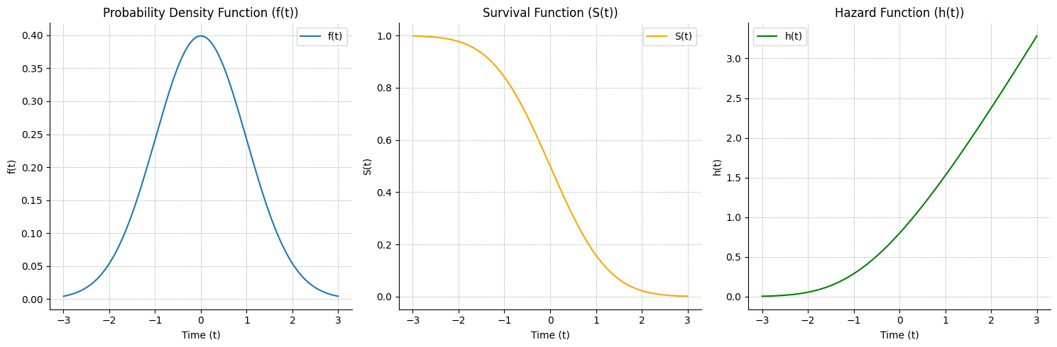
Kurt Vonnegut’s “shape of stories” is entertaining but inaccurate. Hamlet would need an exponential \(f(t)\) to produce the \(h(t)=k\) he described. That would mean that as the plot, for whatever its worth, progresses, there’s an exponentially increasing likelihood of revenge. So do great works have this distribution? that “things” generally happen later than sooner? Inevitability? Damn it. He’s right. We see it with “No Country for Old Men”
Autoencoder
Art must be critiqued
More remote overtones of the harmonic series “heard”?
Embracing of these as inseperable from earlier overtones?
How, then, do our favorite artists perform with regard to one specific overtone?
Best of art uses history:
Reverence
Inference
Deliverance
Case: Bach’s
AirMy
reverencefor him is increased by itYet its mostly my new
inferencesabout music in general that dominate my experienceFrom this vantage I’m in better position to critique and provide much needed
deliverancefrom the shackles of my earlier exposures to music & genres