Black-Scholes#
Efficient-Market Hypothesis#
where:
       1. Chaos
               \
  2. Frenzy -> 4. Unpredictable -> 5. Algorithm -> 6. Binary
               /
               3. Random-Walk

Black-Scholes-Merton. Call option price is analogous to the difference between the base-case & clinical-scenario; i.e., logHR. In clinical medicine, we’ve kept our cumulative distribution functions non-parametric, at least for our base-case (62,000 citations: Google Scholar) 64 65. Here, \(C\) is the call option price, \(S_0\) is the current stock price, \(X\) is the strike price, \(r\) is the risk-free interest rate, \(T\) is the time to maturity, \(\sigma\) is the volatility of the stock, and \(\mathcal{N}(\cdot)\) is the cumulative distribution function of the standard normal distribution.#
ii: Null 1, 2, 3, \(\mu\) Wednesday#
\(f(t)\)
Voir: Random brownian motion as seen in digital information from Bloomberg Terminal; \(\text{H}_0:\)logHR=0\(S(t)\)
Savoir: Compute may find patterns that Eugene Fama’s mind couldn’t\(h(t)\)
Pouvoir: \(\mu | \text{X}\beta\) ; \(\sigma | t\); two overlayed multivariable Kaplan-Meier’s
V7: Sing O Muse 4, \(\sigma\) Year#
\((X'X)^T \cdot X'Y\)
Unpredictable: Estimates conditional on factors millions of orders of magnitude more than human mind “tameth”; no wonder there’s been gnashing of teeth
i: Alternative 5, 6, \(\%\) Tuesday#
\(\beta\)
Identity: Some quants, programmers, and algorithms have produced better returns than the null-hypothesis over decades\(SV_t'\)
Achievements: Using super-humanAIcapabilities of machines to handle \(N^N\) parameters, Jim Simmons is the best way to summarize this
Allusion#
\(S_0\) Base-case#
where:
Show code cell source
# courtesy of meta.ai
import pandas as pd
import numpy as np
from lifelines import KaplanMeierFitter
import matplotlib.pyplot as plt
# Load the data from the CSV file
s0_df = pd.read_csv('~/documents/rhythm/marx/kitabo/ensi/data/s0_nondonor.csv', header=0)
# Create a KaplanMeierFitter object
kmf = KaplanMeierFitter()
# Fit the Kaplan-Meier estimate to the data
kmf.fit(s0_df['_t'], event_observed=s0_df['_d'])
# Get the survival probabilities
survival_probabilities = kmf.survival_function_
# Calculate the failure probabilities (1 - survival probability)
failure_probabilities = 1 - survival_probabilities
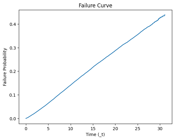
# Plot the failure curve
plt.plot(kmf.timeline, failure_probabilities)
plt.xlabel('Time (_t)')
plt.ylabel('Failure Probability')
plt.title('Failure Curve')
plt.show()
print(s0_df)
Show code cell output
       _st  _d         _t  _t0  s0_nondonor
0        1   1  14.748802    0     0.788091
1        1   0  29.927446    0     0.576725
2        1   0  29.746748    0     0.578996
3        1   0  19.203285    0     0.725669
4        1   0  20.213552    0     0.711040
...    ...  ..        ...  ...          ...
73563    1   0   2.214921    0     0.974868
73564    1   0   1.516769    0     0.983511
73565    1   0   1.415469    0     0.984641
73566    1   0   1.960301    0     0.978229
73567    1   0   1.100616    0     0.988551

[73568 rows x 5 columns]
Model Coefficients#
Show code cell source
b_df = pd.read_csv('../data/b_nondonor.csv', header=0)
print(b_df)
Show code cell output
   A         B  C         D  E         F  G         H         I  J  ...  AW  \
0  0  0.361154  0  0.299617  0 -0.139638  0  0.124114  0.438236  0  ...   0

         AX        AY        AZ        BA        BB        BC       BD  \
0  0.178476  1.200497  0.074832  0.004682 -0.003239  0.000075 -0.00227

         BE        BF
0  0.000005  0.000021

[1 rows x 58 columns]
Show code cell source
import pandas as pd

# Define the meaningless headers and data provided
columns = [
    "A", "B", "C", "D", "E", "F", "G", "H", "I", "J", "K", "L", "M", "N", "O", "P", "Q", "R", "S", "T", "U", "V", "W", "X", "Y", "Z",
    "AA", "AB", "AC", "AD", "AE", "AF", "AG", "AH", "AI", "AJ", "AK", "AL", "AM", "AN", "AO", "AP", "AQ", "AR", "AS", "AT", "AU",
    "AV", "AW", "AX", "AY", "AZ", "BA", "BB", "BC", "BD", "BE", "BF"
]

data = [
    0, 0.3611540640749626, 0, 0.2996174782817143, 0, -0.1396380267801064, 0, 0.1241139571516237, 0.438236411976324, 0,
    -0.059895226414333, 0, 0.3752078798205875, 0, 0.0927075946775824, -0.0744371973326359, 0.1240852498460039, -0.0176059111708996,
    -0.0684981196640994, -0.1339078132620516, -0.1688485989105275, -0.1749309513874832, -0.232756397671939, 0.0548690007396233,
    0.0072862860322084, -0.3660394524818282, -0.4554416752427064, -0.1691931796222081, -0.0781079363323375, 0.368728384689242, 0,
    -0.5287614160906285, -0.5829729708389515, 0, -0.1041236831513535, -0.5286676823325914, -0.2297292995090682, -0.1657466825095737,
    0, 0.2234811404289921, 0.5530365583277806, -43.66976587951415, 0.6850541632181936, 0.3546286547464611, 0.2927117177058185,
    0.2910135188333163, 0.1551116553040275, 0.1682748362958531, 0, 0.1784756812804011, 1.200496862053446, 0.0748319011956608,
    0.0046824977599823, -0.0032389485781854, 0.0000754693150546, -0.0022698686486925, 5.11669774511e-06, 0.0000213400932172
]

# Create a DataFrame
b_df = pd.DataFrame([data], columns=columns)

# Define the variable names provided
variable_names = [
    "diabetes_no", "diabetes_yes", "insulin_no", "insulin_yes", "dia_pill_no", "dia_pill_yes",
    "hypertension_no", "hypertension_yes", "hypertension_dont_know", "hbp_pill_no", "hbp_pill_yes",
    "smoke_no", "smoke_yes", "income_adjusted_ref", "income_adjusted_5000-9999", "income_adjusted_10000-14999",
    "income_adjusted_15000", "income_adjusted_20000", "income_adjusted_25000", "income_adjusted_35000",
    "income_adjusted_45000", "income_adjusted_55000", "income_adjusted_65000-74999", "income_adjusted_>20000",
    "income_adjusted_<20000", "income_adjusted_14", "income_adjusted_15", "refused_to_answer", "dont_know",
    "gender_female", "gender_male", "race_white", "race_mexican_american", "race_other_hispanic",
    "race_non_hispanic_black", "race_other", "hs_good", "hs_excellent", "hs_very_good", "hs_fair", "hs_poor",
    "hs_refused", "hs_8", "hs_dont_know", "education_ref_none", "education_k8", "education_some_high_school",
    "education_high_school", "education_some_college", "education_more_than_college", "education_refused",
    "age_centered", "boxcar_new_centered", "bmi_centered", "egfr_centered", "uacr_centered", "ghp"
]

# Add an additional label to match the number of columns in the DataFrame
variable_names.append("extra_label")

# Apply the variable names to the DataFrame
b_df.columns = variable_nam

# Display the DataFrame
print(b_df)
Show code cell output
   diabetes_no  diabetes_yes  insulin_no  insulin_yes  dia_pill_no  \
0            0      0.361154           0     0.299617            0

   dia_pill_yes  hypertension_no  hypertension_yes  hypertension_dont_know  \
0     -0.139638                0          0.124114                0.438236

   hbp_pill_no  ...  education_some_college  education_more_than_college  \
0            0  ...                       0                     0.178476

   education_refused  age_centered  boxcar_new_centered  bmi_centered  \
0           1.200497      0.074832             0.004682     -0.003239

   egfr_centered  uacr_centered       ghp  extra_label
0       0.000075       -0.00227  0.000005     0.000021

[1 rows x 58 columns]
Scenario Vector#
Show code cell source
SV_df = pd.read_csv('../data/SV_nondonor.csv', header=0)
print(SV_df)
Show code cell output
   SV_nondonor1  SV_nondonor2  SV_nondonor3  SV_nondonor4  SV_nondonor5  \
0             1             0             1             0             0

   SV_nondonor6  SV_nondonor7  SV_nondonor8  SV_nondonor9  SV_nondonor10  ...  \
0             1             1             0             0              1  ...

   SV_nondonor49  SV_nondonor50  SV_nondonor51  SV_nondonor52  SV_nondonor53  \
0              0              1              0            -20              0

   SV_nondonor54  SV_nondonor55  SV_nondonor56  SV_nondonor57  SV_nondonor58
0              0              0             30              0              0

[1 rows x 58 columns]
Show code cell source
import pandas as pd
import numpy as np
import matplotlib.pyplot as plt
# Step 1: Read the CSV files
SV_df = pd.read_csv('~/documents/rhythm/marx/kitabo/ensi/data/SV_nondonor.csv', header=0)
coefficients_df = pd.read_csv('~/documents/rhythm/marx/kitabo/ensi/data//b_nondonor.csv', header=0)
s0_df = pd.read_csv('~/documents/rhythm/marx/kitabo/ensi/data/s0_nondonor.csv', header=0)
# Step 2: Apply the variable names to the scenario vector and coefficient vector
variable_names = [
"diabetes_no", "diabetes_yes", "insulin_no", "insulin_yes", "dia_pill_no", "dia_pill_yes",
"hypertension_no", "hypertension_yes", "hypertension_dont_know", "hbp_pill_no", "hbp_pill_yes",
"smoke_no", "smoke_yes", "income_adjusted_ref", "income_adjusted_5000-9999", "income_adjusted_10000-14999",
"income_adjusted_15000", "income_adjusted_20000", "income_adjusted_25000", "income_adjusted_35000",
"income_adjusted_45000", "income_adjusted_55000", "income_adjusted_65000-74999", "income_adjusted_>20000",
"income_adjusted_<20000", "income_adjusted_14", "income_adjusted_15", "refused_to_answer", "dont_know",
"gender_female", "gender_male", "race_white", "race_mexican_american", "race_other_hispanic",
"race_non_hispanic_black", "race_other", "hs_good", "hs_excellent", "hs_very_good", "hs_fair", "hs_poor",
"hs_refused", "hs_8", "hs_dont_know", "education_ref_none", "education_k8", "education_some_high_school",
"education_high_school", "education_some_college", "education_more_than_college", "education_refused",
"age_centered", "boxcar_new_centered", "bmi_centered", "egfr_centered", "uacr_centered", "ghp"
]
variable_names.append("extra_label")
SV_df.columns = variable_names
coefficients_df.columns = variable_names
# Step 3: Compute the scenario survival probabilities
scenario = SV_df.iloc[0].values
coefficients = coefficients_df.iloc[0].values
log_hazard_ratio = np.dot(scenario, coefficients)
baseline_hazard = -np.log(s0_df['s0_nondonor'])
scenario_hazard = baseline_hazard * np.exp(log_hazard_ratio)
# Step 4: Convert survival probabilities to failure probabilities
baseline_failure = 1 - s0_df['s0_nondonor']
scenario_failure = 1 - np.exp(-scenario_hazard)
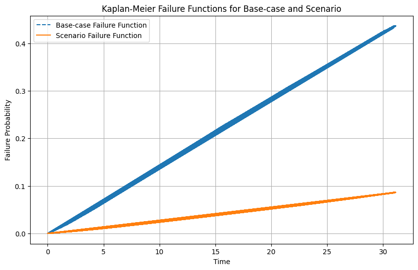
# Step 5: Plot the failure functions
plt.figure(figsize=(10, 6))
plt.plot(s0_df['_t'], baseline_failure, label='Base-case Failure Function', linestyle='--')
plt.plot(s0_df['_t'], scenario_failure, label='Scenario Failure Function', linestyle='-')
plt.xlabel('Time')
plt.ylabel('Failure Probability')
plt.title('Kaplan-Meier Failure Functions for Base-case and Scenario')
plt.legend()
plt.grid(True)
plt.show()

Power dynamics with Salome. Maintaining cheerfulness in the midst of a gloomy task, fraught with immeasurable responsibility, is no small feat; and yet what is needed more than cheerfulnenss? Nothing succeeds if prankishness has no part in it. Excess strength alone is hte proof of strength. 66#