Content with notebooks#
You can also create content with Jupyter Notebooks. This means that you can include code blocks and their outputs in your book.
Markdown + notebooks#
As it is markdown, you can embed images, HTML, etc into your posts!
![]()
You can also \(add_{math}\) and
or
But make sure you $Escape $your $dollar signs $you want to keep!
MyST markdown#
MyST markdown works in Jupyter Notebooks as well. For more information about MyST markdown, check out the MyST guide in Jupyter Book, or see the MyST markdown documentation.
Code blocks and outputs#
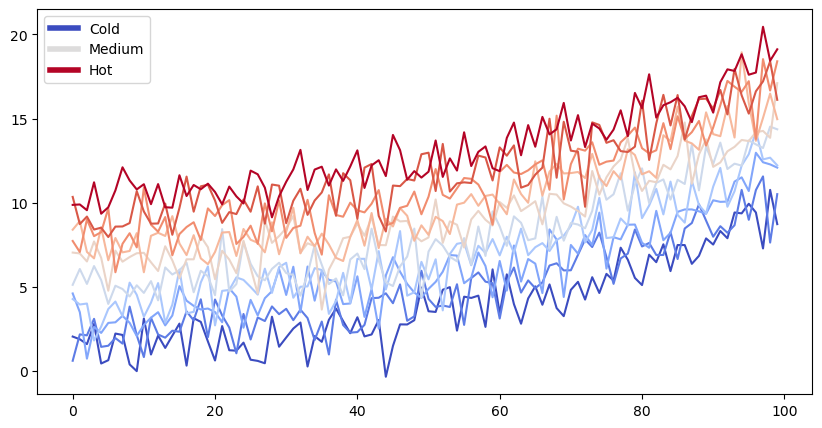
Jupyter Book will also embed your code blocks and output in your book. For example, here’s some sample Matplotlib code:
from matplotlib import rcParams, cycler
import matplotlib.pyplot as plt
import numpy as np
from scipy import stats
import pandas as pd

plt.ion()
<contextlib.ExitStack at 0x103c6b690>
# Fixing random state for reproducibility
np.random.seed(19680801)

N = 10
data = [np.logspace(0, 1, 100) + np.random.randn(100) + ii for ii in range(N)]
data = np.array(data).T
cmap = plt.cm.coolwarm
rcParams['axes.prop_cycle'] = cycler(color=cmap(np.linspace(0, 1, N)))


from matplotlib.lines import Line2D
custom_lines = [Line2D([0], [0], color=cmap(0.), lw=4),
                Line2D([0], [0], color=cmap(.5), lw=4),
                Line2D([0], [0], color=cmap(1.), lw=4)]

fig, ax = plt.subplots(figsize=(10, 5))
lines = ax.plot(data)
ax.legend(custom_lines, ['Cold', 'Medium', 'Hot']);
There is a lot more that you can do with outputs (such as including interactive outputs) with your book. For more information about this, see the Jupyter Book documentation
import numpy as np
import matplotlib.pyplot as plt
from scipy import stats
import pandas as pd
# Load data without specifying data types initially
df = pd.read_csv('~/documents/github/csv/donor_live.csv', low_memory=False)
# Print DataFrame info to verify load
print(df.info())
# Clean and convert data types
df['pers_id'] = pd.to_numeric(df['pers_id'], errors='coerce')
df['don_age_in_months'] = pd.to_numeric(df['don_age_in_months'], errors='coerce')
df['don_age'] = pd.to_numeric(df['don_age'], errors='coerce')
df['don_race'] = pd.to_numeric(df['don_race'], errors='coerce')
# Display basic statistics for continuous variables
print(df[['don_age_in_months', 'don_age', 'don_race']].describe())
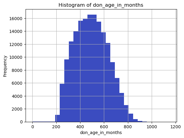
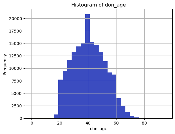
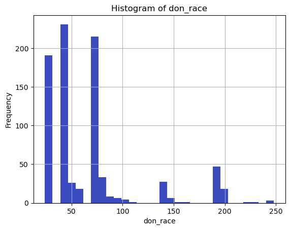
# Plot histograms for continuous variables
continuous_vars = ['don_age_in_months', 'don_age', 'don_race']
for var in continuous_vars:
plt.figure()
df[var].dropna().hist(bins=30)
plt.title(f'Histogram of {var}')
plt.xlabel(var)
plt.ylabel('Frequency')
plt.show()
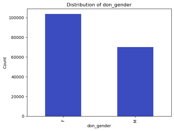
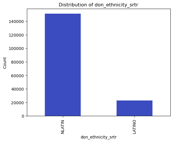
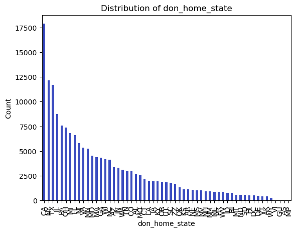
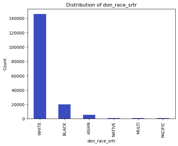
# Count and plot binary/categorical variables
binary_vars = ['don_gender', 'don_ethnicity_srtr']
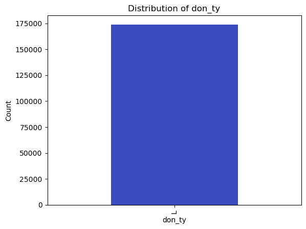
categorical_vars = ['don_ty', 'don_home_state', 'don_race_srtr']
for var in binary_vars + categorical_vars:
plt.figure()
df[var].value_counts().plot(kind='bar')
plt.title(f'Distribution of {var}')
plt.xlabel(var)
plt.ylabel('Count')
plt.show()
<class 'pandas.core.frame.DataFrame'>
RangeIndex: 173929 entries, 0 to 173928
Data columns (total 36 columns):
 #   Column                           Non-Null Count   Dtype
---  ------                           --------------   -----
 0   don_id                           173929 non-null  object
 1   pers_id                          173929 non-null  int64
 2   don_ty                           173929 non-null  object
 3   don_age_in_months                173922 non-null  float64
 4   don_age                          173922 non-null  float64
 5   don_gender                       173929 non-null  object
 6   don_home_state                   170492 non-null  object
 7   don_ethnicity_pre2004            131260 non-null  float64
 8   don_race_pre2004                 131260 non-null  float64
 9   don_race                         173851 non-null  object
 10  don_race_srtr                    173815 non-null  object
 11  don_ethnicity_srtr               173929 non-null  object
 12  don_home_country                 0 non-null       float64
 13  don_hgt_cm                       130924 non-null  float64
 14  don_wgt_kg                       132825 non-null  float64
 15  don_recov_dt                     173929 non-null  object
 16  don_relationship_ty              172919 non-null  object
 17  don_diab                         101127 non-null  object
 18  don_hyperten_diet                3283 non-null    object
 19  don_hyperten_diuretics           3283 non-null    object
 20  don_hyperten_other_meds          3283 non-null    object
 21  don_ki_creat_preop               128276 non-null  float64
 22  don_bp_preop_syst                118935 non-null  float64
 23  don_bp_preop_diast               118915 non-null  float64
 24  pers_esrd_death_dt               79 non-null      float64
 25  pers_ssa_death_dt                1395 non-null    object
 26  don_hyperten_postop              101066 non-null  object
 27  pers_esrd_first_service_dt       706 non-null     float64
 28  pers_esrd_first_dial_dt          690 non-null     float64
 29  pers_esrd_ki_dgn                 332 non-null     float64
 30  don_race_american_indian         173929 non-null  int64
 31  don_race_asian                   173929 non-null  int64
 32  don_race_black_african_american  173929 non-null  int64
 33  don_race_hispanic_latino         173929 non-null  int64
 34  don_race_native_hawaiian         173929 non-null  int64
 35  don_race_white                   173929 non-null  int64
dtypes: float64(14), int64(7), object(15)
memory usage: 47.8+ MB
None
       don_age_in_months        don_age    don_race
count      173922.000000  173922.000000  838.000000
mean          493.620244      40.676142   65.250597
std           139.174427      11.600951   48.149922
min             0.000000       0.000000   24.000000
25%           385.000000      32.000000   40.000000
50%           489.000000      40.000000   40.000000
75%           595.000000      49.000000   72.000000
max          1151.000000      95.000000  248.000000
# Read the CSV file into a DataFrame
df = pd.read_csv('~/documents/github/csv/donor_live.csv')

# Show the DataFrame
You can find the dimensions of a DataFrame using the .shape attribute. This attribute returns a tuple representing the dimensions of the DataFrame, where the first element is the number of rows and the second is the number of columns.
Here’s how to find the dimensions of your DataFrame df:
# Get the dimensions of the DataFrame
rows, cols = df.shape

# Print the dimensions
print(f"The DataFrame has {rows} rows and {cols} columns.")
The DataFrame has 173929 rows and 36 columns.
This will give you a quick idea of how large your dataset is.
Next, you can use the .head() method to print the first 5 rows of your DataFrame. This is a good way to get a feel for what information is in your dataset. You can pass a number into the .head() method to print a different number of rows. For example, df.head(10) will print the first 10 rows of your DataFrame.
df.head()
| don_id | pers_id | don_ty | don_age_in_months | don_age | don_gender | don_home_state | don_ethnicity_pre2004 | don_race_pre2004 | don_race | ... | don_hyperten_postop | pers_esrd_first_service_dt | pers_esrd_first_dial_dt | pers_esrd_ki_dgn | don_race_american_indian | don_race_asian | don_race_black_african_american | don_race_hispanic_latino | don_race_native_hawaiian | don_race_white | |
|---|---|---|---|---|---|---|---|---|---|---|---|---|---|---|---|---|---|---|---|---|---|
| 0 | HRG962 | 289 | L | 490.0 | 40.0 | F | TX | 2.0 | 8.0 | 8: White | ... | N | NaN | NaN | NaN | 0 | 0 | 0 | 0 | 0 | 1 |
| 1 | IT5273 | 484 | L | 312.0 | 26.0 | F | OH | 2.0 | 8.0 | 8: White | ... | N | NaN | NaN | NaN | 0 | 0 | 0 | 0 | 0 | 1 |
| 2 | HRL860 | 840 | L | 648.0 | 54.0 | M | ND | 2.0 | 8.0 | 8: White | ... | N | NaN | NaN | NaN | 0 | 0 | 0 | 0 | 0 | 1 |
| 3 | ZWB847 | 967 | L | 564.0 | 47.0 | M | NY | 1.0 | 8.0 | 2000: Hispanic/Latino | ... | NaN | NaN | NaN | NaN | 0 | 0 | 0 | 1 | 0 | 0 |
| 4 | ALB852 | 1145 | L | 326.0 | 27.0 | F | CA | 1.0 | 8.0 | 2000: Hispanic/Latino | ... | NaN | NaN | NaN | NaN | 0 | 0 | 0 | 1 | 0 | 0 |
5 rows × 36 columns
You can restrict the DataFrame to a subset of rows and columns using slicing. Here’s how to keep only the first 1000 rows and the first 9 columns:
# Subset the DataFrame
subset_df = df.iloc[:1000, :9]

# Show the shape of the new DataFrame to confirm
print(f"The shape of the subset DataFrame is {subset_df.shape}")
The shape of the subset DataFrame is (1000, 9)
Explanation:
df.iloc[:1000, :9]uses theilocindexer for Pandas DataFrames. The:1000selects the first 1000 rows and the:9selects the first 9 columns.subset_df.shapewill display the shape of the new DataFrame, which should be (1000, 9) to confirm that you’ve correctly subsetted it.
Now subset_df contains only the first 1000 rows and the first 9 columns of the original df.
subset_df.head()
| don_id | pers_id | don_ty | don_age_in_months | don_age | don_gender | don_home_state | don_ethnicity_pre2004 | don_race_pre2004 | |
|---|---|---|---|---|---|---|---|---|---|
| 0 | HRG962 | 289 | L | 490.0 | 40.0 | F | TX | 2.0 | 8.0 |
| 1 | IT5273 | 484 | L | 312.0 | 26.0 | F | OH | 2.0 | 8.0 |
| 2 | HRL860 | 840 | L | 648.0 | 54.0 | M | ND | 2.0 | 8.0 |
| 3 | ZWB847 | 967 | L | 564.0 | 47.0 | M | NY | 1.0 | 8.0 |
| 4 | ALB852 | 1145 | L | 326.0 | 27.0 | F | CA | 1.0 | 8.0 |
# Select the first 100 rows and cherry-pick columns by index (e.g., columns at index 0, 2, 4, and 6)
subset_csv = df.iloc[:100, [3, 4, 6]]
subset_csv.to_csv('~/documents/github/work/subset.csv', index=False)
# Summary statistics to identify continuous variables
cont_summary = subset_df.describe()
print("Continuous Variables:")
print(cont_summary.columns.tolist())  # These are likely to be continuous variables

# Identify binary variables
binary_vars = [col for col in subset_df.columns if subset_df[col].nunique() == 2]
print("\nBinary Variables:")
print(binary_vars)

# Identify categorical variables
cat_vars = [col for col in subset_df.select_dtypes(include=['object']).columns if col not in binary_vars]
print("\nCategorical Variables:")
print(cat_vars)
Continuous Variables:
['pers_id', 'don_age_in_months', 'don_age', 'don_ethnicity_pre2004', 'don_race_pre2004']

Binary Variables:
['don_gender', 'don_ethnicity_pre2004']

Categorical Variables:
['don_id', 'don_ty', 'don_home_state']
import numpy as np
import matplotlib.pyplot as plt
from scipy import stats
# Sample data (replace with your own)
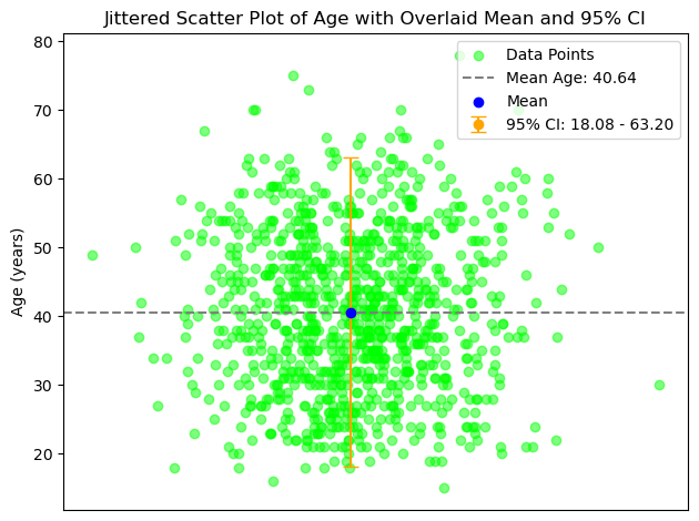
ages = subset_df['don_age'].dropna() # Remove NaN values if any
# Add jitter to x-values for visualization
np.random.seed(42)
jitter = np.random.normal(0, 0.1, len(ages))
# Scatter plot
plt.scatter(jitter, ages, color='lime', alpha=0.5, label='Data Points')
# Calculate mean and 95% CI for ages
mean_age = np.mean(ages)
confidence = 0.95
std_dev = np.std(ages)
ci = std_dev * stats.t.ppf((1 + confidence) / 2, len(ages) - 1)
# Overlay mean as a horizontal line (in gray)
plt.axhline(y=mean_age, color='gray', linestyle='--', label=f'Mean Age: {mean_age:.2f}')
# Overlay mean as a blue dot
plt.scatter(0, mean_age, color='blue', zorder=5, label='Mean')
# Overlay 95% CI as a vertical error bar (in orange)
plt.errorbar(0, mean_age, yerr=ci, color='orange', fmt='o', capsize=5, label=f'95% CI: {mean_age - ci:.2f} - {mean_age + ci:.2f}')
# Remove x-axis ticks, labels, and title
plt.xticks([])
plt.xlabel('')
plt.ylabel('Age (years)')
plt.title('Jittered Scatter Plot of Age with Overlaid Mean and 95% CI')
plt.legend()
plt.tight_layout()
plt.show()